How Can I Learn Excel? Master Excel Skills in 12 Steps

Microsoft Excel stands as a cornerstone of business software worldwide. Its robust capabilities and continuous updates make it an indispensable tool across industries. Whether you’re aiming to boost your career prospects, enhance your data analysis skills, or simply streamline your workflow, learning Excel is a powerful step forward.

This guide provides a clear, 12-step roadmap on How Can I Learn Excel effectively and efficiently. By following these tips and tricks, you’ll not only grasp the fundamentals but also delve into advanced techniques, ultimately impressing colleagues and supervisors alike with your Excel proficiency. Let’s embark on this journey to master Excel and unlock its full potential.

1. Familiarize Yourself with the Excel Interface

If you’re wondering how can I learn excel, the first step is getting comfortable with its layout. Navigating the Excel interface is fundamental to your learning journey.

Let’s begin with basic data entry navigation. When you’re inputting data into Excel, use the Tab key to move to the next cell horizontally, in the column to the right. This is particularly useful for entering data across rows efficiently.

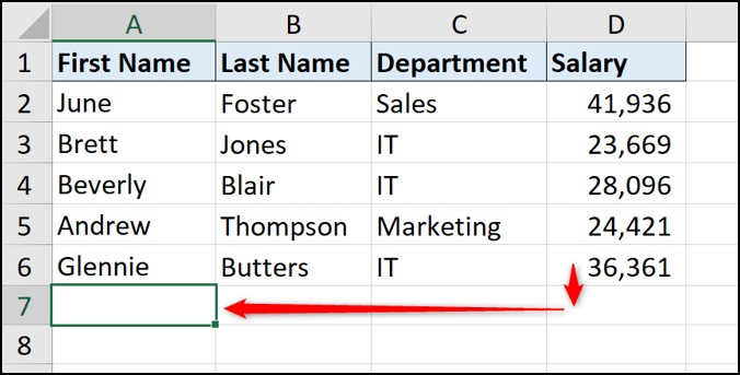
To move vertically down to the next row, simply press Enter. If you’ve been using Tab to navigate across columns, pressing Enter will bring you down one row and back to the starting column, streamlining data entry in columns.

For navigating larger datasets, mastering keyboard shortcuts is crucial. Pressing the Ctrl key in combination with the Up, Down, Left, or Right directional arrow keys will swiftly move you to the last used cell in the respective direction. This is invaluable for quickly jumping to the edges of your data ranges.

To immediately return to the first cell of your dataset, press Ctrl and the Home key together. This shortcut is perfect for quickly orienting yourself within a large spreadsheet. Understanding these basic navigation techniques is a key element in learning excel effectively.

2. Master Essential Excel Shortcuts

To truly accelerate your Excel proficiency, learning and utilizing shortcuts is paramount. These shortcuts, whether keyboard-based or mouse/touchpad actions, drastically reduce the time spent on common tasks, making you a more efficient Excel user.

For beginners asking “how can I learn excel faster?”, start with fundamental keyboard shortcuts. Copying (Ctrl + C) and pasting (Ctrl + V) are universal and essential. The undo command (Ctrl + Z) is a lifesaver for correcting mistakes quickly. Integrating these into your workflow will immediately enhance your speed.

As you become more comfortable, expand your repertoire of Excel shortcuts. Two particularly useful ones are Ctrl + ; to instantly insert today’s date into a cell, and double-clicking the fill handle (the small square at the bottom-right of a selected cell) to rapidly copy cell contents down an entire list.

Excel boasts over 500 keyboard shortcuts, alongside numerous mouse tricks that can significantly speed up your work. While memorizing them all isn’t necessary, learning those that align with your frequent tasks is an excellent strategy for anyone looking to learn excel efficiently.

For those eager to begin using shortcuts, many resources offer printable cheat sheets that can serve as handy references, helping you integrate these time-saving actions into your daily Excel usage.

3. Utilize Freeze Panes for Enhanced Data Visibility

Freeze Panes is an indispensable Excel feature that significantly improves data handling and readability, especially when working with large datasets. Understanding how to use Freeze Panes is a crucial skill when learning excel, as it allows you to keep headers and labels visible, no matter how far you scroll.

Typically, spreadsheet headings reside in the top row. To freeze just the top row, navigate to the View tab on the Excel ribbon, then click Freeze Panes and select Freeze Top Row. This simple action ensures that as you scroll down through your data, the top row containing your headers remains ثابت.

Imagine reviewing data in row 1259; with the top row frozen, your headings are still clearly visible, providing context to the data you’re examining.

Beyond just the top row, Excel allows you to freeze multiple rows and columns. To freeze a specific number of rows and columns, select the cell that is immediately below the rows and to the right of the columns you wish to freeze. For instance, to freeze the first 3 rows and the first column, you would select cell B4.

After selecting the appropriate cell, go to View > Freeze Panes and choose the first Freeze Panes option.

Now, when you scroll down, rows 1, 2, and 3 will remain ثابت. Similarly, if you scroll to the right, column A will stay visible. This is invaluable for maintaining context and understanding data relationships in large spreadsheets.

Mastering Freeze Panes is essential for anyone serious about learning excel, as it greatly enhances efficiency in data review and analysis.

4. Grasp the Power of Excel Formulas

Formulas are the engine of Excel, and becoming proficient in writing them is a cornerstone of mastering Excel. If you are asking how can I learn excel to an advanced level, formulas are your answer. They enable you to perform calculations, manipulate data, and automate tasks, distinguishing proficient users from beginners.

Start with the basics: understand how to create simple formulas for addition, subtraction, multiplication, and division directly within cells. Practice using operators like +, -, *, and / to perform calculations.

Next, delve into commonly used functions. Functions like SUM, IF, VLOOKUP, COUNTIF, and CONCATENATE are frequently used in various Excel tasks. SUM adds ranges of numbers, IF performs logical comparisons, VLOOKUP searches for values in a table, COUNTIF counts cells based on criteria, and CONCATENATE joins text strings.

Once you’re comfortable with these, you’ll realize the immense power formulas provide. You can even integrate formulas into more advanced Excel features like Conditional Formatting and charts, making them dynamic and responsive to data changes.

Exploring available resources that list and explain essential Excel formulas and functions is a great way to expand your knowledge and skills in this critical area. Understanding and utilizing formulas effectively is a key differentiator in learning excel and achieving mastery.

5. Create Simple Drop-Down Lists for Efficient Data Entry

Excel drop-down lists streamline data entry and enhance data accuracy, making them a valuable tool for anyone learning excel. By restricting entries to predefined options, drop-down lists minimize errors and ensure consistency in your spreadsheets.

To create a drop-down list in Excel, follow these steps:

1. Select the Cell Range: First, select the cells where you want the drop-down lists to appear. This could be a single cell or a range of cells.

2. Access Data Validation: Navigate to the Data tab on the Excel ribbon, then click on Data Validation. This will open the Data Validation dialog box.

3. Choose List Validation: In the Data Validation dialog, under the Settings tab, find the Allow dropdown menu. Select List from this menu. This specifies that you want to create a drop-down list.

4. Define the Source: In the Source box, you have two options:

   • Type List Items Directly: Enter the items for your drop-down list, separated by commas (e.g., Option 1,Option 2,Option 3).
   • Select a Cell Range: Alternatively, if your list items are already in a range of cells on your spreadsheet, click the icon to the right of the Source box and select the range containing your list items. This is preferable for longer lists or lists that might need updating.

Once configured, each cell in your selected range will have a drop-down arrow. Clicking this arrow reveals the list of items you defined, allowing users to select an option instead of typing it manually. This feature significantly simplifies data entry, improves accuracy, and is an essential skill to acquire when learning excel.

6. Visualize Data with Conditional Formatting

Conditional Formatting is a powerful Excel feature that allows you to automatically format cells based on specific criteria. It’s a visual tool that quickly highlights key data trends and patterns, making it easier to interpret and analyze information. For anyone learning excel, mastering conditional formatting is essential for effective data visualization.

With Conditional Formatting, you can set rules to automatically change cell colors, add icons, or apply data bars based on values, deadlines, or any other conditions you define. This enables you to instantly see which values meet certain thresholds, such as sales targets, overdue dates, or low inventory levels.

For a simple example, let’s say you want to highlight all values greater than 300 in green. Here’s how:

1. Select the Target Range: Begin by selecting the range of cells to which you want to apply conditional formatting.

2. Access Conditional Formatting: Go to the Home tab on the Excel ribbon, click on Conditional Formatting, then navigate to Highlight Cells Rules, and select Greater Than….

3. Set the Rule: In the ‘Greater Than’ dialog box, enter 300 in the field provided. Then, choose the formatting style you want to apply from the dropdown menu. You can select from predefined formats or customize your own.

In this example, a green fill with dark green text is chosen. Excel offers a variety of formatting options, including font styles, borders, and fill colors.

Beyond simple highlighting, Conditional Formatting in Excel also allows for the application of data bars and icon sets. These visual elements can be very effective in providing a quick, at-a-glance understanding of data distributions and performance metrics. The image below shows data bars applied to the same range of values, providing a visual representation of each value’s magnitude relative to others.

Conditional formatting is a dynamic feature that updates automatically as data changes, making it an invaluable tool for real-time data analysis and monitoring, and a key skill for anyone learning excel for data-driven tasks.

7. Speed Up Data Tasks with Flash Fill

Flash Fill is an intelligent Excel feature designed to automatically recognize patterns in your data and complete tasks for you, significantly speeding up data manipulation. This feature is a game-changer for routine data cleaning and formatting tasks that previously required complex formulas or macros. For those looking at how can I learn excel to enhance productivity, Flash Fill is a must-know.

Consider a scenario where you have a list of full names in one column, and you need to extract just the first names into another column. Traditionally, this might involve using text functions. However, with Flash Fill, the process is incredibly simple.

To use Flash Fill for this task:

1. Start Pattern Recognition: In the column next to your list of full names (e.g., column B), manually type the first name from the first cell (e.g., in cell B2, type “John”). Then, in the cell below (B3), start typing the first name from the second cell (“Jane”).

2. Flash Fill Activation: As you begin typing the second name, Flash Fill detects the pattern of extracting the first name from the adjacent column. Excel will then display a preview of how it will complete the rest of the column based on this pattern.

3. Apply Flash Fill: If the preview looks correct, simply press Enter to accept Flash Fill’s suggestion. Excel will automatically populate the rest of the column with the extracted first names based on the pattern it recognized.

Besides manual initiation by typing, Flash Fill can also be activated through the Excel ribbon. You can find the Flash Fill button in the Data tab, under the Data Tools group. Alternatively, the keyboard shortcut Ctrl + E can also be used to invoke Flash Fill.

Flash Fill is versatile and can be used for various data manipulation tasks such as splitting names, combining data, reformatting dates, and more. Its ease of use and efficiency make it a powerful tool for anyone learning excel, especially those dealing with data cleaning and preparation.

8. Tell Stories Visually with Charts and Graphs

Representing numerical data visually through charts and graphs is a crucial skill for effective communication and analysis in Excel. If you want to know how can I learn excel to present data effectively, mastering data visualization is key. Charts transform raw data into understandable visual stories, highlighting trends, comparisons, and patterns that might be missed in rows and columns of numbers.

Here’s a straightforward 3-step process to create a graph in Excel:

1. Select Your Data: Begin by highlighting the data you want to include in your chart. Ensure your selection includes both the data values and their corresponding labels (like categories or dates).

2. Insert Chart: Go to the Insert tab on the Excel ribbon. In the Charts group, you’ll see various chart types available (e.g., Column, Line, Pie, Bar). Choose the chart type that best suits your data and the story you want to tell. For example, column charts are great for comparing categories, while line charts are effective for showing trends over time.

3. Customize Your Chart: Once inserted, your chart is highly customizable. Excel provides extensive options to modify chart elements like titles, axes labels, legends, colors, and styles.

Chart Customization

Excel’s chart customization capabilities are virtually limitless, allowing you to tailor your visuals precisely. When you select a chart, the Chart Design and Format tabs appear on the ribbon, providing contextual tools for customization.

Using the Chart Design tab, you can quickly change chart styles, switch data sources, alter the chart type, and add or remove chart elements such as titles, legends, data labels, and axis titles.

If you decide that a different chart type might better represent your data, you can easily change it. For example, if you initially chose a bar chart but think a line chart would better illustrate a trend, you can switch types with just a few clicks.

Effective use of charts and graphs transforms data into compelling visual narratives, making complex information accessible and engaging. Mastering Excel charting tools is indispensable for anyone aiming to communicate data insights effectively.

9. Summarize Data Efficiently with PivotTables

PivotTables are among the most powerful features in Excel, designed for summarizing and analyzing large datasets with remarkable ease. If you are exploring how can I learn excel for data analysis, PivotTables are a critical tool to master. They allow you to quickly reorganize and summarize data to extract meaningful insights without writing complex formulas.

Imagine you have a massive sales dataset and need to understand sales performance by region, product category, or time period. PivotTables can break down this data in seconds, showing you sales figures categorized in various ways, such as sales by region, or sales of specific products within each region.

Creating a PivotTable involves a few simple steps:

1. Select Your Data Range: Click anywhere within your dataset. Excel will automatically detect the surrounding data range. It’s best if your data is organized in a tabular format with headers.

2. Insert PivotTable: Go to the Insert tab on the Excel ribbon and click on PivotTable. This opens the ‘Create PivotTable’ dialog box.

3. Configure PivotTable Settings: In the ‘Create PivotTable’ dialog, confirm that the selected range is correct. Choose whether you want to place the PivotTable in a ‘New Worksheet’ or an ‘Existing Worksheet’. Selecting ‘New Worksheet’ is generally recommended for clarity.

4. Build Your PivotTable: Once created, a blank PivotTable structure appears along with the ‘PivotTable Fields’ pane. This pane lists all the column headers from your dataset. To build your report, simply drag and drop fields from this list into the four PivotTable areas: Filters, Columns, Rows, and Values.

   • Columns: Fields placed here become column labels in your PivotTable.
   • Rows: Fields in this area become row labels.
   • Values: Typically numeric fields that you want to summarize (e.g., sum, average, count). Excel automatically applies ‘Sum’ for numeric fields but this can be changed.
   • Filters: Allow you to filter the entire PivotTable based on the selected field.

In the example below, ‘Year’ is dragged to ‘Columns’, ‘Product Category’ to ‘Rows’, and ‘Sales Value’ to ‘Values’. This configuration will display total sales value for each product category, broken down by year.

The ‘Values’ area is where calculations are performed. By default, Excel often uses ‘Sum’, but you can change this to ‘Average’, ‘Count’, ‘Max’, ‘Min’, etc. To change the calculation type, right-click on any value in the PivotTable, select Summarize Values By, and choose your desired function.

PivotTables are incredibly versatile and offer many more advanced features beyond the scope of this basic introduction. However, the best way to learn PivotTables is to experiment. Load up some spreadsheet data, insert a PivotTable, and start dragging fields into different areas to explore the various summarization and analysis options. Hands-on practice is key to truly understanding and mastering PivotTables as part of your Excel learning journey.

10. Protect Your Worksheet Data Integrity

Data accuracy is paramount in Excel, especially when using features like PivotTables, formulas, and conditional formatting. These tools rely on correct data to function effectively. While features like drop-down lists and Flash Fill help maintain data entry accuracy, protecting your data from accidental or unauthorized changes is another critical step in ensuring data integrity. Learning how to protect worksheets is an important aspect of how can I learn excel for professional use.

Excel offers various levels of protection, with sheet protection being the most commonly used. Sheet protection allows you to lock specific cells to prevent modifications while leaving others editable. This is particularly useful in shared workbooks where you want to control which parts of the sheet users can alter.

Protecting a worksheet involves a two-stage process:

1. Unlock Cells for Editing: By default, all cells in an Excel worksheet are locked. Therefore, the first step is to unlock the cells that you want users to be able to edit.

   • Select the range of cells you want to unlock. To select multiple non-contiguous ranges, hold down the Ctrl key while selecting.
   • Press Ctrl + 1 to open the Format Cells dialog box.
   • Go to the Protection tab and uncheck the Locked box. Click OK.

2. Activate Sheet Protection: Once you’ve unlocked the editable cells, you can apply sheet protection.

   • Navigate to the Review tab on the Excel ribbon and click on Protect Sheet.
   • In the ‘Protect Sheet’ dialog box, you can optionally set a password to prevent unprotection (though this is often skipped for simple protection against accidental changes).
   • Select the permissions you want to allow users to have, such as ‘Select locked cells’ and ‘Select unlocked cells’. You can also allow actions like ‘Format cells’ or ‘Insert rows’ if needed. Click OK.

After protection is enabled, users can only edit the cells you unlocked. If they attempt to modify a locked cell, Excel will display a warning message indicating that the sheet is protected and changes are not allowed. This ensures that critical data and formulas remain intact, enhancing the reliability of your spreadsheets.

11. Elevate Your Skills with Power Query and Power Pivot

For users aiming to transcend basic Excel capabilities and delve into advanced data handling and analysis, Power Query and Power Pivot are transformative tools. Mastering these power tools will significantly elevate your Excel skills beyond that of a typical user. For those asking how can I learn excel for data analysis, these are crucial next steps.

Power Query is primarily a data transformation and data preparation tool. Integrated into Excel under the Data tab (Get & Transform Data group), Power Query allows you to import data from a vast array of sources—including files (CSV, Excel, text), databases, web pages, and cloud services. Its capabilities are constantly expanding to include more data sources.

Once data is imported, Power Query Editor provides a user-friendly interface to clean and shape your data. Common operations include:

• Filtering and Sorting: Removing irrelevant data and ordering rows.
• Data Type Conversion: Ensuring columns are in the correct format (e.g., text, number, date).
• Splitting and Merging Columns: Separating data into more useful parts or combining data from multiple columns.
• Removing Duplicates: Ensuring data uniqueness.
• Pivoting and Unpivoting Data: Restructuring data for better analysis.

Power Query records each transformation step you apply. These steps are written in a language called “M,” but you don’t need to learn M to use Power Query effectively for most tasks—the graphical interface handles 99% of common needs. The beauty of Power Query is that once you’ve set up your queries, you can refresh them to pull in the latest data with just a click, automating repetitive data preparation tasks.

Power Pivot, also known as the Data Model, is designed for handling large volumes of data and building complex data models directly within Excel. Unlike standard Excel worksheets which have row limitations, Power Pivot can handle millions of rows, overcoming Excel’s physical limitations.

In Power Pivot, you can:

• Load Large Datasets: Import and manage massive datasets that exceed Excel’s row limits.
• Create Relationships: Define relationships between multiple tables, similar to database relationships, allowing you to combine data from different sources effectively.
• DAX Functions: Use Data Analysis Expressions (DAX) to perform complex calculations across related tables. DAX is more powerful and flexible than standard Excel formulas for data analysis in a data model context.

Power Pivot enables you to perform sophisticated data analysis, create robust reports, and build interactive dashboards, all within Excel. It’s an essential tool for anyone dealing with substantial data volumes or needing to conduct advanced analytical tasks.

12. Automate Tasks with Macros and VBA

Macros in Excel and VBA (Visual Basic for Applications) provide powerful automation capabilities, allowing you to streamline repetitive tasks and significantly boost your productivity. If you’re serious about how can I learn excel to maximize efficiency, automation through macros is a crucial advanced skill.

Macros are essentially recorded sequences of actions that you can replay with a single click or shortcut. They are ideal for automating tasks you perform frequently, saving you time and reducing errors. VBA is the programming language behind Excel macros, offering even greater control and flexibility in automation.

Getting started with macros is surprisingly easy through recording:

1. Access Macro Recorder: Go to the View tab on the Excel ribbon. On the far right, you’ll find the Macros dropdown menu. Click on it and select Record Macro.

2. Record Your Actions: In the ‘Record Macro’ dialog, give your macro a name, assign a shortcut key (optional), and choose where to store the macro. Then, click OK to start recording. From this point, Excel records every action you take—every click, every keystroke. Perform the task you want to automate (e.g., formatting a report, inserting standard text, running a series of calculations).

3. Stop Recording: Once you’ve completed the task, go back to the View tab, Macros dropdown, and click Stop Recording. Your macro is now created.

To run your recorded macro, you can either use the shortcut key you assigned or go to View > Macros > View Macros, select your macro, and click Run.

For more complex automation and customization, you can delve into VBA. To view and edit the VBA code of a recorded macro:

1. View VBA Code: Go to View > Macros > View Macros, select your macro from the list, and click Edit. This opens the VBA editor (Visual Basic for Applications).

In the VBA editor, you can see the code generated by the macro recorder and manually edit or write VBA code to create more sophisticated automation solutions. Learning VBA expands your ability to automate tasks far beyond simple recording, enabling you to create custom functions, control Excel features programmatically, and build interactive Excel applications.

Ready to Master Excel?

While these 12 steps provide a comprehensive guide on how can I learn excel, the most effective approach is structured learning and consistent practice. Consider enrolling in a structured online Excel course that offers a step-by-step curriculum, expert guidance, and hands-on exercises. Practice alongside experienced instructors, like Microsoft MVPs, to gain practical skills and stay updated with the latest Excel features.

[ Level up your Excel skills

Become a certified Excel ninja with GoSkills bite-sized courses

Start free trial ](https://www.goskills.com/Course/Excel?source=blog-cta&blogId=290)

By combining structured learning with continuous practice, you’ll not only master Excel but also unlock its vast potential to enhance your efficiency and productivity in any professional setting.

Join the Excel conversation on Slack! Join Slack channel

Alan Murray
Microsoft Excel MVP, Excel Trainer, and Consultant.

Connect with Alan on LinkedIn