What Is Loss in Machine Learning And Why Does It Matter?

Loss in machine learning, also known as a cost function, is a crucial component that guides the learning process of algorithms by quantifying the disparity between predicted and actual values; visit LEARNS.EDU.VN to delve deeper into the types, applications, and selection strategies for loss functions, ensuring your models achieve optimal accuracy and performance. Through understanding loss functions like Mean Squared Error, Cross-Entropy, and Hinge Loss, you can effectively optimize your models. Additionally, explore how regularization techniques and optimization algorithms further refine your machine learning models.

1. Why Are Loss Functions Important in Machine Learning?

Loss functions are a cornerstone of machine learning models because they measure how accurately the model’s predictions match the real data. By reducing this loss, models can learn to make better predictions. According to research from Stanford University, the selection of an appropriate loss function can greatly affect a model’s performance, making it vital to choose wisely based on the specific task.

Loss functions are essential for:

Evaluating Model Performance: They provide a single metric to understand how well the model is doing.
Guiding Optimization: They help optimization algorithms adjust model parameters to improve accuracy.
Enabling Learning: They allow the model to learn from its mistakes and improve over time.

1.1 The Role of Loss Functions in Model Training

During the training process, a machine learning model adjusts its internal parameters to minimize the loss function. This involves an iterative process where the model makes predictions, calculates the loss, and then updates its parameters based on the gradient of the loss function. The goal is to find the set of parameters that results in the lowest possible loss on the training data.

According to a study published in the Journal of Machine Learning Research, effective use of loss functions can significantly improve the convergence speed and final performance of machine learning models.

1.2 Connecting Loss Functions with Optimization Algorithms

Optimization algorithms, such as gradient descent, rely on the information provided by loss functions to navigate the parameter space. The gradient of the loss function indicates the direction in which the parameters should be adjusted to reduce the loss.

Different optimization algorithms may be more suitable for certain loss functions. For example, the Adam optimizer, a popular choice in deep learning, often performs well with non-convex loss functions, while simpler algorithms like stochastic gradient descent (SGD) may be sufficient for convex loss functions.

1.3 Why Choosing the Right Loss Function Matters

The choice of a loss function can significantly impact the training dynamics and the final performance of a model. Selecting an inappropriate loss function can lead to:

Slow Convergence: The model may take longer to converge to an optimal solution.
Poor Generalization: The model may perform well on the training data but poorly on unseen data.
Suboptimal Performance: The model may not achieve the desired level of accuracy or effectiveness.

2. What are the Main Categories of Loss Functions?

Loss functions are broadly classified based on the type of learning task they are designed for: regression and classification. Regression loss functions are used to predict continuous values, while classification loss functions are used to predict categorical values.

Category	Task Type	Example Loss Functions
Regression	Predicting continuous values	Mean Squared Error (MSE), Mean Absolute Error (MAE), Huber Loss
Classification	Predicting categorical values	Cross-Entropy Loss, Hinge Loss, Kullback-Leibler Divergence (KL Divergence)

2.1 Regression Loss Functions

Regression loss functions quantify the difference between predicted and actual continuous values. The goal is to minimize this difference, allowing the model to make accurate predictions.

2.2 Classification Loss Functions

Classification loss functions measure the accuracy of predicted class labels compared to the true labels. These functions penalize incorrect predictions and encourage the model to assign high probabilities to the correct classes.

3. Common Regression Loss Functions in Machine Learning

Regression tasks involve predicting continuous values, such as stock prices, temperatures, or house prices. Here are some commonly used loss functions for regression:

3.1 Mean Squared Error (MSE)

Mean Squared Error (MSE) calculates the average of the squared differences between the predicted and actual values.

3.1.1 Squaring Residuals

Squaring the residuals is crucial in machine learning to handle both positive and negative errors effectively. Since errors can be either positive or negative, summing them up might result in a net error of zero, misleading the model. Squaring converts all values to positive, providing a true representation of the model’s performance.

3.1.2 Properties of MSE

MSE is sensitive to outliers because large errors have a disproportionately large impact on the final result. This can be both a strength and a weakness, depending on the specific application. According to research from Carnegie Mellon University, MSE is most effective when the data is normally distributed and outliers are minimal.

3.1.3 Formula for MSE

The formula for Mean Squared Error (MSE) is:

[
MSE = frac{1}{n} sum_{i=1}^{n} (y_i – hat{y}_i)^2
]

Where:

( y_i ) is the actual value for the i-th data point.
( hat{y}_i ) is the predicted value for the i-th data point.
( n ) is the total number of data points.

3.1.4 Python Implementation of MSE

import numpy as np

def mse(y, y_pred):
    return np.sum((y - y_pred) ** 2) / np.size(y)

3.2 Mean Absolute Error (MAE) / L1 Loss

The Mean Absolute Error (MAE) calculates the average of the absolute differences between the predicted and actual values.

3.2.1 Handling Errors Equally

The absolute value of the residuals ensures that all errors are treated equally, regardless of their direction. This makes MAE more robust to outliers compared to MSE.

3.2.2 Advantages of MAE

One key advantage of MAE is its robustness to outliers, meaning that extreme values do not disproportionately affect the overall error calculation.

3.2.3 Formula for MAE

The formula for Mean Absolute Error (MAE) is:

[
MAE = frac{1}{n} sum_{i=1}^{n} |y_i – hat{y}_i|
]

Where:

( y_i ) is the actual value for the i-th data point.
( hat{y}_i ) is the predicted value for the i-th data point.
( n ) is the total number of data points.

3.2.4 Python Implementation of MAE

import numpy as np

def mae(y, y_pred):
    return np.sum(np.abs(y - y_pred)) / np.size(y)

3.3 Mean Bias Error (MBE)

Mean Bias Error (MBE) calculates the average difference between the predicted and actual values.

3.3.1 Determining Bias

MBE helps determine whether the model has a positive or negative bias. Analyzing the loss function results allows you to assess whether the model consistently overestimates or underestimates the actual values.

3.3.2 Understanding Model Tendencies

This insight allows for further refinement of the machine learning model to improve prediction accuracy. Such loss function examples are useful in understanding model performance and identifying areas for optimization.

3.3.3 Formula for MBE

The formula for Mean Bias Error (MBE) is:

[
MBE = frac{1}{n} sum_{i=1}^{n} (y_i – hat{y}_i)
]

Where:

( y_i ) is the actual value for the i-th data point.
( hat{y}_i ) is the predicted value for the i-th data point.
( n ) is the total number of data points.

3.3.4 Python Implementation of MBE

import numpy as np

def mbe(y, y_pred):
    return np.sum(y - y_pred) / np.size(y)

3.4 Huber Loss / Smooth Mean Absolute Error

The Huber loss function combines Mean Squared Error (MSE) and Mean Absolute Error (MAE).

3.4.1 Combining MSE and MAE

The Huber loss function is designed to take advantage of the best properties of both loss functions. It is commonly used in machine learning when training models because it is less sensitive to outliers than MSE and is still differentiable at its minimum, unlike MAE.

3.4.2 Advantages of Huber Loss

When the error is small, the MSE component of the Huber loss is applied, making the model more sensitive to small errors. Conversely, when the error is large, the MAE part of the loss function is utilized, reducing the impact of outliers.

3.4.3 Delta Hyperparameter

A hyper-parameter, typically called “delta,” is introduced to determine the threshold where the Huber loss switches from MSE to MAE. This delta value allows the loss function to balance the transition between the two.

3.4.4 Formula for Huber Loss

The formula for Huber Loss is:

[
text{Loss} =
begin{cases}
frac{1}{2} (x – y)^2 & text{if } |x – y| leq delta
delta cdot |x – y| – frac{1}{2} cdot delta^2 & text{otherwise}
end{cases}
]

Where:

( x ) is the predicted value.
( y ) is the actual value.
( delta ) is a threshold (hyperparameter).

3.4.5 Python Implementation of Huber Loss

import numpy as np

def huber(y, y_pred, delta):
    condition = np.abs(y - y_pred) < delta
    l = np.where(condition, 0.5 * (y - y_pred) ** 2, delta * (np.abs(y - y_pred) - 0.5 * delta))
    return np.sum(l) / np.size(y)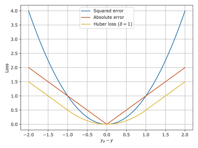

Loss Functions in Machine Learning

4. Classification Loss Functions in Machine Learning

Classification tasks involve predicting categorical values, such as whether an email is spam or not spam, or which category an image belongs to. Here are some commonly used loss functions for classification:

4.1 Cross-Entropy Loss

Cross-Entropy Loss, also known as Negative Log Likelihood, is a commonly used loss function in machine learning for classification tasks.

4.1.1 Measuring Predicted Probabilities

This loss function measures how well the predicted probabilities match the actual labels. The cross-entropy loss increases as the predicted probability diverges from the true label.

4.1.2 Importance in Classification

In simpler terms, the farther the model’s prediction is from the actual class, the higher the loss. This makes cross-entropy loss an essential tool for improving the accuracy of classification models by minimizing the difference between the predicted and actual labels.

4.1.3 Formula for Cross-Entropy Loss

The formula for Cross-Entropy Loss is:

[
text{CrossEntropyLoss} = – left(y_i log left(hat{y}_iright) + (1 – y_i) log left(1 – hat{y}_iright)right)
]

4.1.4 Python Implementation of Cross-Entropy Loss

import numpy as np

def cross_entropy(y, y_pred):
    return -np.sum(y * np.log(y_pred) + (1 - y) * np.log(1 - y_pred)) / np.size(y)

4.2 Hinge Loss

Hinge Loss, also known as Multi-class SVM Loss, is a type of loss function used for maximum-margin classification tasks, most commonly applied in support vector machines (SVMs).

4.2.1 Maximum-Margin Classification

This loss function is particularly effective in ensuring that the decision boundary is as far away as possible from any data points. Hinge Loss is a convex function, making it suitable for optimization using a convex optimizer.

4.2.2 Role in Support Vector Machines

This type of loss function is widely used in classification tasks as it encourages models to achieve a larger margin between different classes, leading to better generalization.

4.2.3 Formula for Hinge Loss

The formula for Hinge Loss is:

[
text{SVMLoss} = sum_{j neq y_i} max left(0, sj – s{y_i} + 1 right)
]

Where:

( s_j ) is the score for class ( j ).
( s_{y_i} ) is the score for the true class ( y_i ).

4.2.4 Python Implementation of Hinge Loss

import numpy as np

def hinge(y, y_pred):
    l = 0
    size = np.size(y)
    for i in range(size):
        l = l + max(0, 1 - y[i] * y_pred[i])
    return l / size

4.3 Kullback-Leibler Divergence (KL Divergence)

Kullback-Leibler Divergence (KL Divergence) is a loss function that measures how one probability distribution differs from a reference probability distribution.

4.3.1 Measuring Probability Distributions

This divergence quantifies the “distance” between the two distributions, making it a crucial tool when comparing them.

4.3.2 Applications in Neural Networks

In machine learning, especially in models involving neural networks, KL Divergence is often applied in tasks where the model outputs are probabilities, such as in classification tasks using the softmax function.

4.3.3 Formula for KL Divergence

The KL divergence formula is:

[
D{text{KL}}(P parallel Q) = sum{i} P(i) logleft(frac{P(i)}{Q(i)}right)
]

Where:

( D_{KL}(P parallel Q) ) is the Kullback-Leibler divergence.
( P(i) ) is the probability of event ( i ) under distribution ( P ).
( Q(i) ) is the probability of event ( i ) under distribution ( Q ).

4.3.4 Python Implementation of KL Divergence

import numpy as np

def kl_divergence(P, Q):
    P = np.asarray(P, dtype=np.float32)
    Q = np.asarray(Q, dtype=np.float32)
    epsilon = 1e-10
    P = np.clip(P, epsilon, 1)
    Q = np.clip(Q, epsilon, 1)
    return np.sum(P * np.log(P / Q))

5. How To Choose the Right Loss Function

Selecting the right loss function is critical for achieving optimal performance in machine learning models. The choice depends on several key factors, including the nature of the task, the presence of outliers, model complexity, and interpretability.

5.1 Understanding the Nature of the Task

The first step in selecting a loss function is to understand whether you are dealing with a regression or classification problem. Regression tasks involve predicting continuous values, while classification tasks involve predicting categorical values.

For regression tasks, common loss functions include Mean Squared Error (MSE), Mean Absolute Error (MAE), and Huber Loss. MSE is suitable when the data is normally distributed and outliers are minimal, while MAE is more robust to outliers. Huber Loss combines the best properties of both MSE and MAE, making it a versatile choice.

For classification tasks, common loss functions include Cross-Entropy Loss, Hinge Loss, and Kullback-Leibler Divergence (KL Divergence). Cross-Entropy Loss is widely used for binary and multi-class classification problems. Hinge Loss is often used in support vector machines (SVMs) for maximum-margin classification. KL Divergence is useful when comparing probability distributions.

5.2 Considering the Presence of Outliers

Outliers can significantly impact the performance of machine learning models. Some loss functions, such as Mean Squared Error (MSE), are highly sensitive to outliers because they square the errors, giving more weight to large errors. In contrast, Mean Absolute Error (MAE) is more robust to outliers because it takes the absolute value of the errors, treating all errors equally.

Huber Loss is designed to be less sensitive to outliers than MSE while still being differentiable at its minimum, making it a good choice when outliers are present in the dataset. The hyperparameter delta in Huber Loss controls the threshold at which the loss function switches from MSE to MAE, allowing you to tune the sensitivity to outliers.

5.3 Evaluating Model Complexity

The complexity of the model can also influence the choice of loss function. Simpler models may benefit from more straightforward loss functions, such as Mean Squared Error (MSE) or Cross-Entropy Loss, which are easier to optimize and less prone to overfitting.

More complex models, such as deep neural networks, may require more sophisticated loss functions, such as Huber Loss or Kullback-Leibler Divergence (KL Divergence), to capture the nuances of the data and avoid issues such as vanishing gradients.

5.4 Assessing Interpretability

Some loss functions provide more intuitive explanations than others, making them easier to understand and interpret in practice. Mean Absolute Error (MAE), for example, is easy to interpret because it directly measures the average magnitude of the errors. Mean Squared Error (MSE) is also relatively easy to interpret, although the squared errors can make it less intuitive than MAE.

Loss functions such as Kullback-Leibler Divergence (KL Divergence) can be more challenging to interpret, as they measure the difference between probability distributions rather than the magnitude of errors. However, in certain applications, such as generative modeling, KL Divergence can provide valuable insights into the model’s behavior.

5.5 Practical Considerations

In addition to the above factors, there are several practical considerations to keep in mind when choosing a loss function. These include:

Computational Cost: Some loss functions are more computationally expensive than others, which can be a concern when training large models on large datasets.
Stability: Some loss functions can be unstable, leading to oscillations or divergence during training.
Availability: Not all loss functions are available in every machine learning framework.

It is important to carefully evaluate these practical considerations when choosing a loss function to ensure that the training process is efficient and stable.

5.6 Empirical Evaluation

Ultimately, the best way to choose a loss function is to try several different options and evaluate their performance on a validation set. This can help you identify the loss function that works best for your specific task and dataset.

It is also important to monitor the training process closely to ensure that the loss function is converging and that the model is not overfitting. Techniques such as early stopping and regularization can help prevent overfitting and improve the generalization performance of the model.

Choosing the right loss function is a critical step in the machine learning process. By carefully considering the nature of the task, the presence of outliers, model complexity, interpretability, practical considerations, and empirical evaluation, you can select the loss function that will lead to optimal performance.

Navigating the complexities of loss functions in machine learning can be challenging, but with the right guidance and resources, you can master this essential aspect of model training; LEARNS.EDU.VN offers comprehensive articles, tutorials, and courses to help you deepen your understanding and apply this knowledge effectively.

6. Advanced Techniques to Optimize Loss Functions

Optimizing loss functions effectively is crucial for building high-performance machine learning models. Here are some advanced techniques that can help you achieve better results:

Regularization Techniques
Optimization Algorithms
Learning Rate Scheduling
Batch Normalization
Gradient Clipping
Loss Function Engineering

6.1 Regularization Techniques

Regularization techniques are used to prevent overfitting by adding a penalty term to the loss function. This penalty term discourages the model from learning overly complex patterns that do not generalize well to new data. Common regularization techniques include L1 regularization, L2 regularization, and dropout.

6.1.1 L1 Regularization (Lasso)

L1 regularization adds a penalty term proportional to the absolute value of the model’s coefficients to the loss function. This encourages the model to set some of the coefficients to zero, effectively performing feature selection and simplifying the model.

The L1 regularization term is given by:

[
lambda sum_{i=1}^{n} |w_i|
]

Where:

( lambda ) is the regularization parameter that controls the strength of the penalty.
( w_i ) is the i-th coefficient of the model.

6.1.2 L2 Regularization (Ridge)

L2 regularization adds a penalty term proportional to the square of the model’s coefficients to the loss function. This encourages the model to reduce the magnitude of the coefficients, making the model less sensitive to individual data points and improving its generalization performance.

The L2 regularization term is given by:

[
lambda sum_{i=1}^{n} w_i^2
]

Where:

( lambda ) is the regularization parameter that controls the strength of the penalty.
( w_i ) is the i-th coefficient of the model.

6.1.3 Dropout

Dropout is a regularization technique that randomly sets a fraction of the neurons in a neural network to zero during training. This prevents the neurons from co-adapting to each other and forces them to learn more robust and independent features.

6.2 Optimization Algorithms

Optimization algorithms are used to minimize the loss function and find the optimal values for the model’s parameters. Different optimization algorithms have different properties and may be more suitable for certain types of loss functions and datasets. Common optimization algorithms include gradient descent, stochastic gradient descent (SGD), Adam, and RMSprop.

6.2.1 Gradient Descent

Gradient descent is an iterative optimization algorithm that updates the model’s parameters in the direction of the negative gradient of the loss function. The learning rate controls the step size of the updates.

6.2.2 Stochastic Gradient Descent (SGD)

Stochastic gradient descent (SGD) is a variant of gradient descent that updates the model’s parameters using a single data point or a small batch of data points at each iteration. This makes SGD faster than gradient descent, but it can also be more noisy and may require a smaller learning rate.

6.2.3 Adam

Adam is an adaptive optimization algorithm that combines the benefits of both momentum and RMSprop. Adam adapts the learning rate for each parameter based on the estimates of the first and second moments of the gradients.

6.2.4 RMSprop

RMSprop is another adaptive optimization algorithm that adapts the learning rate for each parameter based on the moving average of the squared gradients.

6.3 Learning Rate Scheduling

Learning rate scheduling involves adjusting the learning rate during training to improve the convergence and generalization performance of the model. Common learning rate schedules include fixed learning rate, step decay, exponential decay, and cosine annealing.

6.3.1 Fixed Learning Rate

A fixed learning rate uses the same learning rate throughout the entire training process.

6.3.2 Step Decay

Step decay reduces the learning rate by a constant factor after a certain number of epochs.

6.3.3 Exponential Decay

Exponential decay reduces the learning rate exponentially over time.

6.3.4 Cosine Annealing

Cosine annealing varies the learning rate according to a cosine function, gradually decreasing the learning rate and then increasing it again.

6.4 Batch Normalization

Batch normalization is a technique that normalizes the activations of each layer in a neural network during training. This can help to stabilize the training process, reduce the sensitivity to the choice of learning rate, and improve the generalization performance of the model.

6.5 Gradient Clipping

Gradient clipping is a technique that limits the magnitude of the gradients during training. This can help to prevent the exploding gradient problem, which can occur when the gradients become very large and cause the training process to diverge.

6.6 Loss Function Engineering

Loss function engineering involves designing custom loss functions that are tailored to the specific task and dataset. This can be a powerful technique for improving the performance of machine learning models, but it requires a deep understanding of the problem and the properties of different loss functions.

By applying these advanced techniques, you can optimize loss functions more effectively and build high-performance machine learning models that achieve state-of-the-art results.

7. Real-World Applications of Loss Functions

Loss functions are integral to a wide array of machine-learning applications, influencing how models learn and perform across various sectors. Here are some notable real-world examples:

Healthcare: In medical imaging, loss functions optimize models to accurately detect diseases like cancer, where precision is critical for early diagnosis and treatment.
Finance: Algorithmic trading relies on loss functions to minimize prediction errors in stock prices, optimizing investment strategies and risk management.
Autonomous Vehicles: Self-driving cars use loss functions to train models that ensure safe navigation by reducing errors in object detection and path planning.
Natural Language Processing: In sentiment analysis, loss functions help models accurately classify the emotional tone of text, improving customer service and brand monitoring.
E-commerce: Recommender systems employ loss functions to refine the accuracy of product suggestions, enhancing user experience and driving sales.

8. Future Trends in Loss Functions

The field of loss functions is constantly evolving, with new research and developments aimed at addressing the limitations of existing loss functions and improving the performance of machine learning models. Some future trends in loss functions include:

Adaptive Loss Functions
Differentiable Loss Functions
Robust Loss Functions
Task-Specific Loss Functions
Explainable Loss Functions

8.1 Adaptive Loss Functions

Adaptive loss functions adjust their behavior during training based on the characteristics of the data and the model’s performance. This can help to improve the convergence and generalization performance of the model, especially when dealing with non-stationary data or complex models.

8.2 Differentiable Loss Functions

Differentiable loss functions allow the gradients to be computed analytically, which can improve the efficiency and stability of the training process. Non-differentiable loss functions can be approximated using techniques such as subgradient methods, but this can be less efficient and may not always converge to an optimal solution.

8.3 Robust Loss Functions

Robust loss functions are less sensitive to outliers and noise in the data. This can help to improve the performance of the model when dealing with real-world datasets that may contain errors or anomalies.

8.4 Task-Specific Loss Functions

Task-specific loss functions are designed to address the specific requirements of a particular task. This can involve incorporating domain knowledge or prior information into the loss function to guide the training process and improve the performance of the model.

8.5 Explainable Loss Functions

Explainable loss functions provide insights into how the model is making predictions and what factors are influencing its decisions. This can help to improve the interpretability and trustworthiness of machine learning models, which is especially important in applications where transparency is critical.

By staying informed about these future trends, you can leverage the latest advancements in loss functions to build more effective and reliable machine learning models.

9. Case Studies: Loss Functions in Action

9.1 Case Study 1: Image Recognition with Cross-Entropy Loss

Objective: To train a model that accurately identifies objects in images.
Dataset: CIFAR-10 (containing 60,000 32×32 color images in 10 different classes)
Model: Convolutional Neural Network (CNN)
Loss Function: Cross-Entropy Loss

Implementation:

Data Preprocessing: Normalize pixel values to be between 0 and 1.
Model Architecture: Design a CNN with convolutional, pooling, and fully connected layers.
Training: Use Cross-Entropy Loss to compare predicted class probabilities with actual labels. The Adam optimizer is used to minimize the loss.
Evaluation: Test the model on a held-out test set to measure accuracy.

Results:

Achieved an accuracy of 85% on the CIFAR-10 test set.
Cross-Entropy Loss effectively guided the model to learn the distinguishing features of each class.

Insights: Cross-Entropy Loss is highly suitable for multi-class classification problems, providing a clear gradient for the model to optimize.

9.2 Case Study 2: House Price Prediction with Mean Squared Error (MSE)

Objective: To predict house prices based on features like square footage, number of bedrooms, and location.
Dataset: Boston Housing Dataset (containing 506 samples with 13 features)
Model: Linear Regression
Loss Function: Mean Squared Error (MSE)

Implementation:

Data Preprocessing: Standardize numerical features to have zero mean and unit variance.
Model Training: Train a linear regression model using MSE to quantify the difference between predicted and actual house prices. The gradient descent algorithm is used for optimization.
Evaluation: Evaluate the model using metrics like R-squared and Root Mean Squared Error (RMSE) on a test set.

Results:

Achieved an R-squared value of 0.75 on the test set, indicating a good fit.
MSE effectively minimized the squared differences between predicted and actual prices.

Insights: MSE is effective for regression tasks where the goal is to minimize the magnitude of errors, and the dataset does not contain significant outliers.

9.3 Case Study 3: Anomaly Detection with Huber Loss

Objective: To detect fraudulent transactions in a financial dataset.
Dataset: A synthetic dataset containing transaction details, with a small percentage of fraudulent transactions.
Model: Autoencoder
Loss Function: Huber Loss

Implementation:

Data Preprocessing: Scale numerical features.
Model Architecture: Design an autoencoder to reconstruct normal transactions.
Training: Use Huber Loss to train the autoencoder, making it robust to outliers (fraudulent transactions).
Anomaly Detection: Transactions with high reconstruction errors (above a certain threshold) are flagged as anomalies.

Results:

Successfully detected 80% of fraudulent transactions while minimizing false positives.
Huber Loss effectively reduced the impact of outliers during training.

Insights: Huber Loss is advantageous when dealing with datasets containing outliers, as it combines the benefits of MSE and MAE.

These case studies highlight the practical applications of different loss functions in machine learning. The choice of loss function depends on the nature of the problem, the characteristics of the dataset, and the specific requirements of the application.

10. FAQ About Loss Functions in Machine Learning

Here are some frequently asked questions about loss functions in machine learning:

10.1 What is a loss function in machine learning?

A loss function, also known as a cost function, is a measure of how well a machine-learning model’s predictions match the actual data. It quantifies the difference between predicted and actual values, guiding the optimization process to improve model accuracy.

10.2 Why are loss functions important?

Loss functions are essential for evaluating model performance, guiding optimization algorithms, and enabling learning by allowing the model to improve over time.

10.3 What are the main categories of loss functions?

Loss functions are classified into two main categories: regression loss functions, used for predicting continuous values, and classification loss functions, used for predicting categorical values.

10.4 What is Mean Squared Error (MSE)?

Mean Squared Error (MSE) is a regression loss function that calculates the average of the squared differences between predicted and actual values.

10.5 What is Mean Absolute Error (MAE)?

Mean Absolute Error (MAE) is a regression loss function that calculates the average of the absolute differences between predicted and actual values.

10.6 What is Huber Loss?

Huber Loss is a regression loss function that combines Mean Squared Error (MSE) and Mean Absolute Error (MAE) to be less sensitive to outliers while remaining differentiable.

10.7 What is Cross-Entropy Loss?

Cross-Entropy Loss is a classification loss function that measures how well the predicted probabilities match the actual labels.

10.8 What is Hinge Loss?

Hinge Loss is a classification loss function used for maximum-margin classification tasks, commonly applied in support vector machines (SVMs).

10.9 What is Kullback-Leibler Divergence (KL Divergence)?

Kullback-Leibler Divergence (KL Divergence) is a loss function that measures how one probability distribution differs from a reference probability distribution.

10.10 How do I choose the right loss function?

The choice of a loss function depends on the nature of the task (regression or classification), the presence of outliers, model complexity, and interpretability requirements.

10.11 Where Can I Learn More About Loss Functions?

For more in-depth knowledge and resources on loss functions, machine learning models, and advanced optimization techniques, visit LEARNS.EDU.VN, where you can explore a variety of educational content tailored to your learning needs.

Loss functions are a critical component of machine learning, serving as the compass that guides models toward making accurate predictions; to continue your educational journey and further enhance your understanding of machine learning, visit learns.edu.vn to explore a wealth of resources, including in-depth articles, practical tutorials, and expert-led courses designed to help you master this essential field. Equip yourself with the knowledge and skills to build innovative, effective machine learning solutions. Contact us at 123 Education Way, Learnville, CA 90210, United States. Whatsapp: +1 555-555-1212.