Principal Component Analysis (PCA) is a powerful technique used across various machine learning applications. At LEARNS.EDU.VN, we’re dedicated to providing clear and insightful explanations of complex topics. PCA simplifies datasets, enhances model performance, and aids in data visualization. By understanding PCA, you can unlock significant improvements in your machine learning projects. Discover how PCA is the transformative technique that can optimize your models and provide deeper insights into your data through dimensionality reduction techniques and feature extraction.
1. What is Principal Component Analysis (PCA)?
Principal Component Analysis (PCA) is a dimensionality reduction technique commonly used in machine learning. PCA transforms a large set of variables into a smaller one that still contains most of the information in the large set. By reducing the number of variables, PCA simplifies data sets, making them easier to explore, visualize, and analyze. This process helps machine learning algorithms work faster and more efficiently by removing extraneous variables. According to research from the University of California, Berkeley, PCA can significantly reduce the computational load in machine learning tasks while preserving critical data features.
1.1. Understanding Dimensionality Reduction
Dimensionality reduction is a crucial concept in machine learning. It involves reducing the number of variables (or dimensions) in a data set while retaining its essential information. The primary goal is to simplify the data without losing critical patterns or trends. This simplification helps in several ways:
- Improved Model Performance: Reducing the number of variables decreases the complexity of the model, which can prevent overfitting and improve generalization.
- Faster Training Times: Fewer variables mean less computation, leading to quicker model training.
- Enhanced Visualization: It is easier to visualize data in two or three dimensions, allowing for better understanding and insight.
1.2. How PCA Achieves Dimensionality Reduction
PCA achieves dimensionality reduction by identifying the principal components of the data. Principal components are new variables that are constructed as linear combinations of the original variables. These combinations are created in such a way that:
- The new variables (principal components) are uncorrelated.
- Most of the information within the initial variables is compressed into the first few components.
The principal components are ranked by the amount of variance they explain in the data. The first principal component accounts for the largest possible variance, the second accounts for the next highest variance, and so on. By discarding the components with low variance, you can reduce the dimensionality of the data without losing much information.
2. What are Principal Components?
Principal components are new, uncorrelated variables that are linear combinations of the original variables. They capture the most significant patterns in the data, with the first component capturing the most variance, the second capturing the second most, and so on.
2.1. Constructing Principal Components
Principal components are constructed in a way that the first principal component accounts for the largest possible variance in the data set. For example, if you have a scatter plot of your data, the first principal component is approximately the line that goes through the origin and maximizes the variance (the average of the squared distances from the projected points to the origin).
The second principal component is calculated similarly, with the condition that it is uncorrelated (perpendicular) to the first principal component and accounts for the next highest variance. This process continues until a total of p principal components have been calculated, equal to the original number of variables.
2.2. Interpreting Principal Components
One important thing to realize is that principal components are less interpretable and don’t have any real meaning since they are constructed as linear combinations of the initial variables. Geometrically speaking, principal components represent the directions of the data that explain a maximal amount of variance.
Think of principal components as new axes that provide the best angle to see and evaluate the data, so that the differences between the observations are better visible.
3. Key Steps in Performing PCA
To perform PCA, follow these five key steps: standardization, covariance matrix computation, eigenvector and eigenvalue calculation, feature vector creation, and data recasting.
3.1. Step 1: Standardization
The aim of this step is to standardize the range of the continuous initial variables so that each one of them contributes equally to the analysis. It is critical to perform standardization prior to PCA because PCA is sensitive to the variances of the initial variables. Variables with larger ranges will dominate over those with small ranges, leading to biased results.
Mathematically, this can be done by subtracting the mean and dividing by the standard deviation for each value of each variable:
- Formula: z = (x – μ) / σ
- Where:
zis the standardized valuexis the original valueμis the mean of the variableσis the standard deviation of the variable
- Where:
Once the standardization is done, all the variables will be transformed to the same scale.
3.2. Step 2: Covariance Matrix Computation
The aim of this step is to understand how the variables of the input data set are varying from the mean with respect to each other, or in other words, to see if there is any relationship between them. Sometimes, variables are highly correlated in such a way that they contain redundant information. To identify these correlations, compute the covariance matrix.
The covariance matrix is a p × p symmetric matrix (where p is the number of dimensions) that has as entries the covariances associated with all possible pairs of the initial variables. For example, for a 3-dimensional data set with 3 variables x, y, and z, the covariance matrix is a 3×3 data matrix of this form:
| Cov(x,x)  Cov(x,y)  Cov(x,z) |
| Cov(y,x)  Cov(y,y)  Cov(y,z) |
| Cov(z,x)  Cov(z,y)  Cov(z,z) |
Since the covariance of a variable with itself is its variance (Cov(a,a)=Var(a)), in the main diagonal (Top left to bottom right) you actually have the variances of each initial variable. And since the covariance is commutative (Cov(a,b)=Cov(b,a)), the entries of the covariance matrix are symmetric with respect to the main diagonal, which means that the upper and the lower triangular portions are equal.
What do the covariances that you have as entries of the matrix tell us about the correlations between the variables?
It’s actually the sign of the covariance that matters:
- Positive Covariance: The two variables increase or decrease together (correlated).
- Negative Covariance: One variable increases when the other decreases (inversely correlated).
Now that you know that the covariance matrix is not more than a table that summarizes the correlations between all the possible pairs of variables, let’s move to the next step.
3.3. Step 3: Compute Eigenvectors and Eigenvalues
Eigenvectors and eigenvalues are linear algebra concepts that you need to compute from the covariance matrix in order to determine the principal components of the data.
What you first need to know about eigenvectors and eigenvalues is that they always come in pairs, so that every eigenvector has an eigenvalue. Also, their number is equal to the number of dimensions of the data. For example, for a 3-dimensional data set, there are 3 variables, therefore there are 3 eigenvectors with 3 corresponding eigenvalues.
Eigenvectors and eigenvalues are behind all the magic of principal components because the eigenvectors of the Covariance matrix are actually the directions of the axes where there is the most variance (most information) and that we call Principal Components. And eigenvalues are simply the coefficients attached to eigenvectors, which give the amount of variance carried in each Principal Component.
By ranking your eigenvectors in order of their eigenvalues, highest to lowest, you get the principal components in order of significance.
Principal Component Analysis Example:
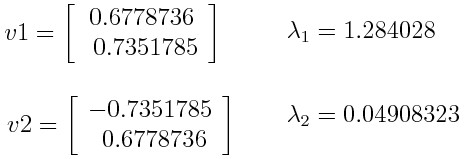
Let’s suppose that your data set is 2-dimensional with 2 variables x,y and that the eigenvectors and eigenvalues of the covariance matrix are as follows:
Eigenvalues: λ1 = 96, λ2 = 4
Eigenvectors: v1 = [0.707, 0.707], v2 = [-0.707, 0.707]
If you rank the eigenvalues in descending order, you get λ1>λ2, which means that the eigenvector that corresponds to the first principal component (PC1) is v1 and the one that corresponds to the second principal component (PC2) is v2.
After having the principal components, to compute the percentage of variance (information) accounted for by each component, you divide the eigenvalue of each component by the sum of eigenvalues. If you apply this on the example above, you find that PC1 and PC2 carry respectively 96 percent and 4 percent of the variance of the data.
3.4. Step 4: Create a Feature Vector
As we saw in the previous step, computing the eigenvectors and ordering them by their eigenvalues in descending order, allow you to find the principal components in order of significance. In this step, what you do is, to choose whether to keep all these components or discard those of lesser significance (of low eigenvalues), and form with the remaining ones a matrix of vectors that you call Feature vector.
So, the feature vector is simply a matrix that has as columns the eigenvectors of the components that you decide to keep. This makes it the first step towards dimensionality reduction, because if you choose to keep only p eigenvectors (components) out of n, the final data set will have only p dimensions.
Principal Component Analysis Example:
Continuing with the example from the previous step, you can either form a feature vector with both of the eigenvectors v1 and v2:
Feature Vector = | 0.707  -0.707 |
                 | 0.707   0.707 |
Or discard the eigenvector v2, which is the one of lesser significance, and form a feature vector with v1 only:
Feature Vector = | 0.707 |
                 | 0.707 |
Discarding the eigenvector v2 will reduce dimensionality by 1, and will consequently cause a loss of information in the final data set. But given that v2 was carrying only 4 percent of the information, the loss will be therefore not important and you will still have 96 percent of the information that is carried by v1.
So, as you saw in the example, it’s up to you to choose whether to keep all the components or discard the ones of lesser significance, depending on what you are looking for. Because if you just want to describe your data in terms of new variables (principal components) that are uncorrelated without seeking to reduce dimensionality, leaving out lesser significant components is not needed.
3.5. Step 5: Recast the Data Along the Principal Components Axes
In the previous steps, apart from standardization, you do not make any changes on the data, you just select the principal components and form the feature vector, but the input data set remains always in terms of the original axes (i.e, in terms of the initial variables).
In this step, which is the last one, the aim is to use the feature vector formed using the eigenvectors of the covariance matrix, to reorient the data from the original axes to the ones represented by the principal components (hence the name Principal Components Analysis). This can be done by multiplying the transpose of the original data set by the transpose of the feature vector.
4. Why Use PCA in Machine Learning?
PCA is used in machine learning to reduce the number of variables in a dataset while preserving important information. This can lead to faster training times, simpler models, and improved visualization.
4.1. Benefits of Using PCA
Using PCA in machine learning offers several benefits:
- Dimensionality Reduction: Reduces the number of variables, simplifying the dataset and reducing computational complexity.
- Noise Reduction: By focusing on the principal components, PCA can filter out noise and irrelevant information.
- Improved Model Performance: Simplifies models, reducing the risk of overfitting and improving generalization.
- Data Visualization: Reduces data to two or three dimensions, making it easier to visualize and understand.
4.2. Applications of PCA
PCA is used in various machine learning applications, including:
- Image Recognition: Reduces the dimensionality of image data, making it easier to identify patterns and features.
- Bioinformatics: Analyzes gene expression data to identify key genes and pathways.
- Finance: Reduces the number of variables in financial models, improving their accuracy and efficiency.
- Data Compression: Compresses data by reducing its dimensionality, saving storage space and bandwidth.
5. PCA and Machine Learning Algorithms
PCA can be used as a preprocessing step for various machine learning algorithms, including linear regression, logistic regression, and support vector machines (SVMs).
5.1. PCA for Linear Regression
In linear regression, PCA can be used to reduce the number of predictors, simplifying the model and reducing the risk of overfitting. By using the principal components as predictors, the model can focus on the most important patterns in the data.
5.2. PCA for Logistic Regression
Similarly, in logistic regression, PCA can be used to reduce the number of features, simplifying the model and improving its generalization performance. This is particularly useful when dealing with high-dimensional data.
5.3. PCA for Support Vector Machines (SVMs)
PCA can also be used to preprocess data for SVMs. By reducing the dimensionality of the data, PCA can speed up the training process and improve the performance of the SVM model, especially when dealing with complex datasets.
6. PCA in Real-World Applications
PCA is applied in various real-world scenarios to simplify data and improve model performance. Let’s explore some specific examples.
6.1. Example 1: Image Compression
PCA can be used to compress images by reducing the number of components needed to represent them. For example, an image can be represented by its principal components, and only the most significant components are stored. This significantly reduces the storage space required while preserving most of the image’s visual information.
6.2. Example 2: Face Recognition
In face recognition, PCA can be used to reduce the dimensionality of facial images, making it easier to identify faces. The principal components, also known as “eigenfaces,” capture the most important features of the faces, allowing for efficient and accurate recognition.
6.3. Example 3: Gene Expression Analysis
In bioinformatics, PCA is used to analyze gene expression data. By reducing the dimensionality of the data, PCA can help identify key genes and pathways that are associated with certain diseases or conditions. This information can be used to develop new treatments and therapies.
7. Practical Tips for Implementing PCA
Implementing PCA effectively requires careful consideration of the data and the specific goals of the analysis. Here are some practical tips to help you get the most out of PCA.
7.1. Data Preprocessing
Before applying PCA, it’s crucial to preprocess the data to ensure that it is suitable for analysis. This typically involves:
- Handling Missing Values: Impute or remove missing values to avoid errors in the PCA calculation.
- Scaling the Data: Standardize or normalize the data to ensure that all variables are on the same scale.
7.2. Choosing the Number of Components
One of the key decisions when using PCA is determining how many principal components to retain. There are several methods for making this decision:
- Variance Explained: Choose the number of components that explain a certain percentage of the variance (e.g., 95%).
- Scree Plot: Look for the “elbow” in the scree plot, where the variance explained by each component starts to level off.
- Cross-Validation: Use cross-validation to evaluate the performance of the model with different numbers of components and choose the number that gives the best performance.
7.3. Interpreting the Results
Once PCA has been performed, it’s important to interpret the results to understand what the principal components represent. This involves:
- Examining the Loadings: Look at the loadings (the coefficients of the linear combinations) to see which original variables contribute most to each principal component.
- Visualizing the Data: Plot the data in terms of the principal components to see if there are any patterns or clusters.
8. Common Mistakes to Avoid When Using PCA
Using PCA effectively requires avoiding common mistakes that can lead to suboptimal results. Here are some pitfalls to watch out for.
8.1. Not Scaling the Data
Failing to scale the data is one of the most common mistakes when using PCA. If the variables are not on the same scale, the principal components will be dominated by the variables with the largest ranges, leading to biased results.
8.2. Retaining Too Few Components
Retaining too few components can result in a significant loss of information, which can negatively impact the performance of the model. Be sure to choose the number of components carefully, using methods like variance explained or cross-validation.
8.3. Misinterpreting the Components
Misinterpreting the principal components can lead to incorrect conclusions. Remember that the principal components are linear combinations of the original variables, and their meaning may not be immediately obvious. Take the time to examine the loadings and understand which variables contribute most to each component.
9. Advanced PCA Techniques
Beyond the standard PCA, there are several advanced techniques that can be used to address specific challenges and improve the results.
9.1. Kernel PCA
Kernel PCA is a non-linear extension of PCA that uses kernel functions to map the data into a higher-dimensional space before performing PCA. This allows Kernel PCA to capture non-linear relationships in the data that standard PCA cannot.
9.2. Sparse PCA
Sparse PCA is a variation of PCA that encourages the loadings to be sparse (i.e., have many zero entries). This makes the principal components easier to interpret and can improve the performance of the model when dealing with high-dimensional data.
9.3. Incremental PCA
Incremental PCA is a version of PCA that can be used to process large datasets that do not fit into memory. It works by processing the data in batches and updating the principal components incrementally.
10. PCA and Data Visualization
PCA is a powerful tool for data visualization, allowing you to reduce high-dimensional data to two or three dimensions, making it easier to visualize and understand.
10.1. Creating PCA Plots
To create a PCA plot, you first perform PCA to reduce the data to two or three principal components. Then, you plot the data points in terms of these components. The resulting plot shows the relationships between the data points in a lower-dimensional space.
10.2. Interpreting PCA Plots
A PCA plot can reveal patterns and clusters in the data that may not be apparent in the original high-dimensional space. For example, data points that are close together in the PCA plot are likely to be similar, while data points that are far apart are likely to be different.
11. PCA vs. Other Dimensionality Reduction Techniques
PCA is just one of many dimensionality reduction techniques available. Let’s compare it to some other popular methods.
11.1. PCA vs. Linear Discriminant Analysis (LDA)
Linear Discriminant Analysis (LDA) is another dimensionality reduction technique that is commonly used in machine learning. While PCA seeks to find the principal components that explain the most variance in the data, LDA seeks to find the linear discriminants that best separate different classes.
11.2. PCA vs. t-Distributed Stochastic Neighbor Embedding (t-SNE)
t-Distributed Stochastic Neighbor Embedding (t-SNE) is a non-linear dimensionality reduction technique that is particularly well-suited for visualizing high-dimensional data. Unlike PCA, which seeks to preserve the global structure of the data, t-SNE seeks to preserve the local structure, making it better at revealing clusters and patterns.
11.3. PCA vs. Autoencoders
Autoencoders are neural networks that can be used for dimensionality reduction. They work by learning a compressed representation of the data in the bottleneck layer of the network. Unlike PCA, autoencoders can capture non-linear relationships in the data.
12. Future Trends in PCA Research
Research on PCA continues to evolve, with new techniques and applications being developed. Here are some of the future trends in PCA research.
12.1. Deep Learning and PCA
Deep learning and PCA are increasingly being combined to create powerful models. For example, PCA can be used to preprocess data for deep learning models, reducing the dimensionality and improving performance. Additionally, deep learning models can be used to learn non-linear principal components.
12.2. PCA for Big Data
With the increasing availability of big data, there is growing interest in developing PCA techniques that can handle large datasets efficiently. Incremental PCA and distributed PCA are two approaches that are being used to address this challenge.
12.3. Interpretable PCA
There is also growing interest in developing PCA techniques that are more interpretable. Sparse PCA and non-negative matrix factorization (NMF) are two approaches that can produce more interpretable components.
13. Conclusion
Principal Component Analysis (PCA) is a versatile and powerful technique for dimensionality reduction in machine learning. By reducing the number of variables while preserving essential information, PCA simplifies datasets, enhances model performance, and aids in data visualization. Understanding the principles and applications of PCA can significantly improve your machine learning projects.
Whether you’re working on image recognition, bioinformatics, finance, or any other data-intensive field, PCA provides a valuable tool for simplifying data and extracting meaningful insights. As you continue to explore machine learning, consider how PCA can help you optimize your models and gain a deeper understanding of your data.
Ready to dive deeper into the world of machine learning and PCA? Visit LEARNS.EDU.VN for more comprehensive guides, courses, and resources. Unlock your potential and transform your data into actionable insights with our expert guidance.
Address: 123 Education Way, Learnville, CA 90210, United States
WhatsApp: +1 555-555-1212
Website: learns.edu.vn
14. Frequently Asked Questions (FAQ)
14.1. What is the primary goal of PCA in machine learning?
The primary goal of PCA in machine learning is to reduce the dimensionality of a dataset while preserving the most important information, simplifying the data for analysis and modeling.
14.2. How does PCA help in improving machine learning model performance?
PCA helps improve model performance by reducing the number of variables, which can prevent overfitting, speed up training times, and enhance generalization.
14.3. What are principal components, and how are they constructed?
Principal components are new, uncorrelated variables that are linear combinations of the original variables. They are constructed in a way that the first component captures the largest possible variance, the second captures the second largest, and so on.
14.4. Why is standardization important before applying PCA?
Standardization is important because PCA is sensitive to the variances of the initial variables. Standardizing the data ensures that each variable contributes equally to the analysis, preventing biased results.
14.5. What is a covariance matrix, and why is it computed in PCA?
A covariance matrix summarizes the correlations between all possible pairs of variables in the dataset. It is computed to understand how the variables vary with respect to each other, helping identify redundant information.
14.6. How do eigenvectors and eigenvalues relate to PCA?
Eigenvectors represent the directions of the axes where there is the most variance (principal components), and eigenvalues represent the amount of variance carried in each principal component.
14.7. What is a feature vector, and how is it used in PCA?
A feature vector is a matrix that has as columns the eigenvectors of the components you decide to keep. It is used to reorient the data from the original axes to the ones represented by the principal components.
14.8. In what real-world applications is PCA used?
PCA is used in various real-world applications, including image compression, face recognition, gene expression analysis, and finance.
14.9. What are some common mistakes to avoid when using PCA?
Common mistakes include not scaling the data, retaining too few components, and misinterpreting the components.
14.10. How can PCA be used for data visualization?
PCA can be used for data visualization by reducing high-dimensional data to two or three dimensions, making it easier to visualize patterns and clusters in the data.