Decision trees are fundamental to machine learning, offering a clear and intuitive approach to predictive modeling. In our previous discussion on decision trees, we explored their basic structure, highlighting how they mimic human decision-making through a tree-like model. Internal nodes represent tests on features, branches signify decision rules, and leaf nodes provide the final predictions. This foundational knowledge is essential for understanding, building, and interpreting decision trees, which are extensively used in both classification and regression tasks.
Building upon this foundation, let’s delve deeper into the implementation of decision trees within machine learning. We will explore the process of training a decision tree model, making predictions, and evaluating its performance, providing a comprehensive understanding of this powerful algorithm.
Why Choose a Decision Tree Structure in ML?
A decision tree is a versatile supervised learning algorithm applicable to both classification and regression problems. Its strength lies in modeling decisions as a tree-like structure. In this structure, internal nodes represent tests on different attributes, branches correspond to the possible values of those attributes, and leaf nodes embody the ultimate decisions or predictions. Decision trees are favored for their interpretability, adaptability, and wide applicability in machine learning for predictive modeling.
Understanding the intuition behind decision trees is crucial before moving forward. Let’s explore this with a simple example.
Unveiling the Intuition Behind Decision Trees
Consider a scenario where you need to decide whether to bring an umbrella when you leave home. A decision tree approach to this would look like this:
- Step 1 – Initial Question (Root Node): Is it currently raining? If the answer is yes, you decide to take an umbrella. If no, you proceed to consider other factors.
- Step 2 – Further Questions (Internal Nodes): Since it’s not raining now, you ask: Is there a forecast of rain later today? If yes, you decide to take an umbrella. If no, you proceed further.
- Step 3 – Final Decision (Leaf Node): Based on your answers to these questions, you reach a final decision: either take the umbrella or leave it behind.
This simple example illustrates the core idea of a decision tree: breaking down complex decisions into a series of simpler, sequential questions.
Decision Tree Approach: Step-by-Step
Decision trees utilize a tree representation to solve problems. Each leaf node in the tree corresponds to a class label, while attributes are represented by the internal nodes. Decision trees are capable of representing any boolean function on discrete attributes.
Example: Predicting Computer Game Preference
Let’s consider predicting whether a person enjoys computer games based on two attributes: age and gender. Here’s how a decision tree would approach this:
- Starting with the Root Question (Age):
- The initial question is: “Is the person younger than 15 years old?”
- If Yes, follow the left branch.
- If No, follow the right branch.
- Branching Based on Age:
- If the person is younger than 15, they are considered likely to enjoy computer games (assigned a prediction score of +2).
- If the person is 15 or older, the next question is asked: “Is the person male?”
- Branching Based on Gender (for those 15+):
- If the person is male, they are moderately likely to enjoy computer games (assigned a prediction score of +0.1).
- If the person is not male, they are less likely to enjoy computer games (assigned a prediction score of -1).
This example can be further expanded using multiple decision trees to refine predictions.
Enhancing Prediction with Multiple Decision Trees
Example: Predicting Computer Game Preference Using Two Decision Trees
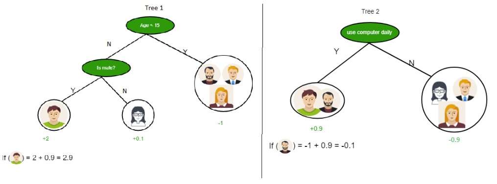
Consider using two decision trees to improve the prediction of computer game preference.
Tree 1: Age and Gender
- This tree uses two questions:
- “Is the person’s age less than 15?”
- If Yes, assign a score of +2.
- If No, proceed to the next question.
- “Is the person male?”
- If Yes, assign a score of +0.1.
- If No, assign a score of -1.
- “Is the person’s age less than 15?”
Tree 2: Computer Usage
- This tree focuses on daily computer usage:
- “Does the person use a computer daily?”
- If Yes, assign a score of +0.9.
- If No, assign a score of -0.9.
- “Does the person use a computer daily?”
Combining Trees for a Final Prediction
The final prediction score is calculated by summing the scores from both trees. This ensemble approach can lead to more robust and accurate predictions.
Attribute Selection Measures: Information Gain and Gini Index
Now that we understand the basic intuition and approach of decision trees, let’s explore the attribute selection measures used in building them. These measures determine which attributes are most effective for splitting the data at each node. Two popular measures are:
- Information Gain
- Gini Index
1. Information Gain:
Information Gain assesses the effectiveness of an attribute in classifying the data. It quantifies the reduction in entropy (uncertainty) achieved by partitioning the data based on a given attribute. A higher Information Gain indicates a more effective attribute for splitting. The attribute with the highest Information Gain is selected as the decision node.
For instance, if splitting a dataset based on ‘age’ into “Young” and “Old” perfectly separates those who bought a product from those who didn’t, the Information Gain is high. This indicates ‘age’ is a highly informative attribute for predicting product purchase in this dataset.
- Let S be a dataset of instances, and A be an attribute. Let Sv be the subset of S where attribute A has value v, and Values(A) be the set of all possible values for attribute A. The Information Gain, Gain(S, A), is calculated as:
[Tex]Gain(S, A) = Entropy(S) – sum_{v epsilon Values(A)}frac{left | S_{v} right |}{left | S right |}. Entropy(S_{v}) [/Tex]
Entropy: Entropy measures the impurity or randomness of a dataset. In the context of decision trees, it quantifies the uncertainty in predicting the class label. Higher entropy indicates greater disorder, while lower entropy indicates more homogeneity.
For example, in a dataset where outcomes are equally split between “Yes” and “No,” entropy is high, reflecting uncertainty. Conversely, if all outcomes are the same (“Yes” or “No”), entropy is zero, indicating no uncertainty.
- The formula for Entropy H(S) of a dataset S is:
[Tex]Entropy(S) = – sum_{i=1}^{c} p_i log_{2} p_i[/Tex]
Where (p_i) is the proportion of instances belonging to class i, and c is the number of classes.
Example Calculation of Entropy:
Consider a set X = {a, a, a, b, b, b, b, b}.
- Total instances: 8
- Instances of ‘b’: 5
- Instances of ‘a’: 3
[Tex]begin{aligned}text{Entropy } H(X) & = -left [ left ( frac{3}{8} right )log_{2}frac{3}{8} + left ( frac{5}{8} right )log_{2}frac{5}{8} right ]\& = -[0.375 (-1.415) + 0.625 (-0.678)] \& = -(-0.53-0.424) \& = 0.954end{aligned}[/Tex]
Building a Decision Tree Using Information Gain: Key Steps
- Start at the Root: Begin with all training instances at the root node.
- Attribute Selection: Use Information Gain to select the best attribute for splitting at each node.
- No Attribute Repetition: Ensure no attribute is repeated along any root-to-leaf path when dealing with discrete attributes.
- Recursive Tree Construction: Recursively build subtrees for each branch, based on the subsets of training instances classified down that path.
- Leaf Node Labeling:
- If all instances in a subset belong to the same class, label the node as that class.
- If no attributes remain for splitting, label the node with the majority class of the remaining instances.
- If a subset is empty, label the node with the majority class from the parent node’s instances.
Example: Decision Tree Construction with Information Gain
Let’s construct a decision tree for the following dataset using Information Gain.
Training Set: 3 Features, 2 Classes
| X | Y | Z | C |
|---|---|---|---|
| 1 | 1 | 1 | I |
| 1 | 1 | 0 | I |
| 0 | 0 | 1 | II |
| 1 | 0 | 0 | II |
Here, we have three features (X, Y, Z) and two classes (I, II). To build the decision tree, we calculate the Information Gain for each feature.
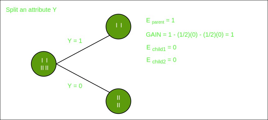
Split on Feature X:
Split on Feature Y:
Split on Feature Z:
Analysis reveals that splitting on Feature Y yields the highest Information Gain. Thus, Feature Y is chosen as the root node. Observing the splits based on Feature Y, we see that the resulting subsets are pure concerning the target variable. Consequently, no further splitting is needed.
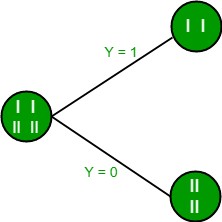
The final decision tree is:
2. Gini Index
The Gini Index measures the impurity of a dataset, indicating the likelihood of misclassifying a randomly chosen element. A lower Gini Index suggests higher purity, making attributes with lower Gini Indices preferable for splitting. Scikit-learn (Sklearn), a popular Python machine learning library, supports “gini” as a criterion for using the Gini Index in decision trees, and it is the default setting.
For example, in a group where everyone bought a product (100% “Yes”), the Gini Index is 0, indicating perfect purity. In contrast, a group with an equal mix of “Yes” and “No” responses will have a Gini Index of 0.5, showing higher impurity or uncertainty.
The formula for the Gini Index is:
[Tex]Gini = 1 – sum_{i=1}^{n} p_i^2[/Tex]
Key Features and Characteristics of the Gini Index:
- Calculation: It is computed by summing the squared probabilities of each class in a dataset and subtracting this sum from 1.
- Purity Indication: A lower Gini Index signifies a more homogeneous distribution, while a higher value indicates a more heterogeneous or impure distribution.
- Decision Tree Application: In decision trees, the Gini Index evaluates split quality by measuring the reduction in impurity from the parent node to the weighted average impurity of the child nodes.
- Computational Efficiency: Compared to entropy, the Gini Index is computationally faster and more sensitive to changes in class probabilities.
- Bias towards Equal-Sized Splits: The Gini Index tends to favor splits that result in equally sized child nodes, which may not always optimize classification accuracy.
- Practical Choice: The choice between using the Gini Index or entropy depends on the specific problem and dataset, often requiring empirical testing and tuning.
Real-world Use Case: Understanding Decision Trees in Action
Let’s walk through a real-life use case to understand how a decision tree works step by step.
Step 1. Start with the Entire Dataset: Begin with the complete dataset, considering it as the root node of the decision tree.
Step 2. Select the Best Attribute (Question): Choose the most informative attribute to partition the dataset. For instance, consider the attribute “Outlook.”
- Possible values for “Outlook”: Sunny, Cloudy, or Rainy.
Step 3. Partition Data into Subsets: Divide the dataset into subsets based on the attribute values:
- Subset for “Sunny” outlook.
- Subset for “Cloudy” outlook.
- Subset for “Rainy” outlook.
Step 4. Recursive Partitioning (Further Splitting if Needed): For each subset, determine if further splitting is necessary to refine the classifications. For example, within the “Sunny” subset, you might ask: “Is humidity high or normal?”
- High humidity → Classify as “Swimming.”
- Normal humidity → Classify as “Hiking.”
Step 5. Assign Final Class Labels (Leaf Nodes): When a subset contains instances of only one class, stop splitting and assign a class label:
- “Cloudy” outlook → Classify as “Hiking.”
- “Rainy” outlook → Classify as “Stay Inside.”
- “Sunny” outlook and “High Humidity” → Classify as “Swimming.”
- “Sunny” outlook and “Normal Humidity” → Classify as “Hiking.”
Step 6. Prediction Using the Decision Tree: To predict the class for a new instance, traverse the decision tree:
- Example: For an instance with “Sunny” outlook and “High” humidity:
- Start at the “Outlook” node.
- Follow the branch for “Sunny.”
- Proceed to the “Humidity” node and follow the branch for “High Humidity.”
- The prediction is “Swimming.”
This process demonstrates how a decision tree iteratively splits data based on attributes, leading to a structured decision-making process.
Conclusion
Decision trees are a vital machine learning tool, adept at modeling and predicting outcomes from input data using a tree-like framework. Their key advantages include interpretability, versatility, and ease of visualization, making them invaluable for both classification and regression tasks. While decision trees are easy to understand and implement, challenges like overfitting need to be addressed. A solid grasp of their terminology and construction process is crucial for effectively applying decision trees in diverse machine learning applications.
Frequently Asked Questions (FAQs)
1. What are the major issues in decision tree learning?
Overfitting is a primary concern, where the tree becomes too complex and fits the training data too closely, reducing its ability to generalize to new data. Other issues include sensitivity to small changes in the data and potential instability. Techniques like pruning, setting constraints on tree depth, and using ensemble methods can help mitigate these issues.
2. How do decision trees aid in decision making?
Decision trees provide a transparent and interpretable model for decision-making. They visually represent the decision process as a series of rules, making it easy to understand how a decision is reached. This interpretability is particularly valuable in applications where understanding the reasoning behind predictions is crucial.
3. What is the maximum depth of a decision tree and why is it important?
The maximum depth is a hyperparameter that limits the number of levels in a decision tree. It is crucial for controlling the complexity of the model. A shallower tree may underfit, failing to capture important patterns, while a deeper tree is prone to overfitting. Tuning the maximum depth is essential for balancing model complexity and generalization performance.
4. What is the fundamental concept behind a decision tree?
The core concept is to recursively partition the dataset into subsets based on the most informative attributes at each step. This process creates a tree-like structure that maps features to outcomes. The goal is to create pure subsets at the leaf nodes, where each subset ideally contains instances of only one class or similar values for regression tasks.
5. What is the role of entropy in decision trees?
Entropy is used to measure the impurity or disorder of a dataset. In decision trees, it helps quantify the uncertainty associated with class labels. The algorithm aims to reduce entropy at each split, selecting attributes that maximize information gain (reduction in entropy) to create more homogeneous subsets.
6. What are the key Hyperparameters of decision trees?
- Max Depth: Controls the maximum depth of the tree.
- Min Samples Split: Specifies the minimum number of samples required to split an internal node.
- Min Samples Leaf: Sets the minimum number of samples required in a leaf node.
- Criterion: Defines the function used to measure the quality of a split (e.g., “gini” for Gini Index, “entropy” for Information Gain).
Next Article KNN vs Decision Tree in Machine Learning
Abhishek Sharma 44
Improve this article if you find anything incorrect by clicking on the “Improve Article” button below.