Ensemble learning techniques have consistently demonstrated their ability to boost the performance of machine learning models across various problems. Whether you’re tackling regression or classification challenges, combining multiple models can lead to more robust and accurate predictions. These techniques aggregate the outputs of several base models to form a final, enhanced prediction, often using methods like averaging, voting, or stacking.
This article delves into the world of ensemble learning, exploring how these powerful methods can be leveraged to create optimal machine learning models. We’ll examine both fundamental and advanced techniques, and discuss how platforms like Neptune AI can aid in managing and optimizing your ensemble learning projects.
Understanding Ensemble Learning
At its core, ensemble learning is about strategically combining multiple machine learning models to solve a single problem. These individual models are frequently referred to as “weak learners.” The fundamental principle is that by intelligently aggregating the predictions of several weak learners, we can construct a “strong learner” that outperforms any single model in the ensemble.
Each weak learner is trained on the dataset and generates its own set of predictions. The magic of ensemble learning lies in how these predictions are combined to produce a final, more accurate result.
Basic Ensemble Learning Techniques
Let’s begin by exploring some of the foundational ensemble learning methods:
Max Voting
In the realm of classification problems, each model’s prediction can be considered a vote. The max voting technique determines the final prediction by selecting the class that receives the majority of votes.
Consider a scenario with three classifiers making the following class predictions:
- Classifier 1: Class A
- Classifier 2: Class B
- Classifier 3: Class B
In this case, the final prediction using max voting would be Class B, as it garnered the most votes.
Averaging
Averaging is primarily used in regression problems. Here, the final prediction is calculated as the simple average of all individual model predictions. For example, in random forest regression, the ultimate prediction is the average of predictions from all the constituent decision trees.
Imagine three regression models predicting the price of a commodity:
- Regressor 1: $200
- Regressor 2: $300
- Regressor 3: $400
The averaged prediction would be the mean of these values, which is $300.
Weighted Averaging
Weighted averaging takes the concept of averaging a step further by assigning different weights to each base model’s prediction. Models with higher predictive accuracy are given greater importance by assigning them larger weights. In the commodity price prediction example, we could assign weights reflecting each regressor’s performance.
Assuming regressors are assigned weights of 0.35, 0.45, and 0.2 respectively (summing to 1), the final prediction would be:
(0.35 $200) + (0.45 $300) + (0.2 * $400) = $285
Advanced Ensemble Learning Techniques
Beyond these basic methods, several advanced ensemble techniques offer more sophisticated ways to combine models and enhance performance:
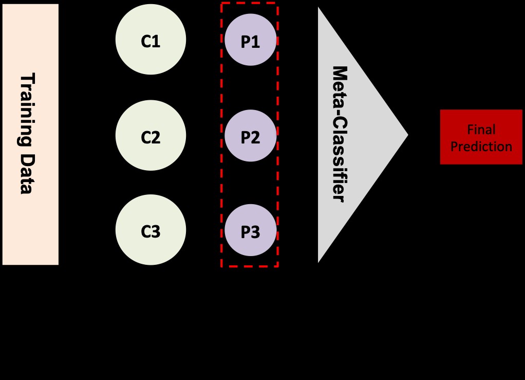
Stacking
Stacking is a method designed to minimize bias by combining diverse estimators. It involves stacking predictions from multiple base estimators and using these stacked predictions as input features for a meta-model (or final estimator). This meta-model is then trained to produce the ultimate prediction. Cross-validation plays a crucial role in training the meta-model.
Stacking is applicable to both regression and classification tasks.
Source: towardsdatascience.com
The stacking process typically unfolds in the following steps:
- Divide your dataset into training and validation sets.
- Further split the training set into K folds (e.g., 10 folds).
- Train a base model (like Support Vector Machines – SVM) on K-1 folds and predict on the held-out fold.
- Repeat step 3 until predictions are generated for all K folds.
- Train the base model on the entire training set.
- Use this trained base model to make predictions on the test set.
- Repeat steps 3-6 for other base models (e.g., decision trees, neural networks).
- Use the predictions from the validation set (from steps 3-4) and the test set (from step 6) as features to train a new meta-model.
- Finally, use the meta-model to generate final predictions on the test set.
For regression problems, the values passed to the meta-model are numerical predictions. For classification, they are usually probabilities or class labels. Tools like Neptune AI can help track and compare the performance of each layer in your stacking ensemble.
Blending
Blending shares similarities with stacking, but it utilizes a holdout set from the training data for predictions. Predictions are made by base models on this holdout set only. These predictions, along with the holdout set, are then used to train a final meta-model which predicts on the test set.
Blending can be viewed as a simplified form of stacking where the meta-model is trained on predictions made by base models on a specific hold-out validation set, rather than through cross-validation.
The blending process generally includes:
- Splitting data into training, validation, and test sets.
- Training base models on the training set.
- Generating predictions on both the validation and test sets using these base models.
- Using the validation set and its corresponding predictions as training data to build and train a meta-model.
- Applying the trained meta-model to the test set predictions to produce final results.
The concept of blending gained prominence during the Netflix Prize competition. The winning team’s solution, which significantly improved Netflix’s recommendation algorithm, was based on a blended approach.
According to a Kaggle ensembling guide, blending is considered a simpler alternative to stacked generalization, reducing the risk of information leakage. Instead of out-of-fold predictions, blending uses a small holdout set (e.g., 10% of the training data) to train the meta-model exclusively.
Blending vs Stacking
While blending is less complex and can prevent information leakage since generalizers and stackers operate on different datasets, it may use less data for training the meta-model, potentially leading to overfitting. Stacking, with its use of cross-validation, generally provides a more robust approach compared to blending, as it leverages more folds for a comprehensive evaluation. Neptune AI can be instrumental in managing the datasets and predictions at each stage of both blending and stacking.
Bagging
Bagging, short for Bootstrap Aggregating, involves creating multiple subsets of the original dataset through random sampling with replacement. For each subset, a base learning algorithm is trained. Bagging then aggregates the predictions from all models, typically using averaging for regression and voting for classification, to produce a generalized prediction.
The bagging method comprises these steps:
- Creating multiple bootstrap samples (random subsets with replacement) from the original dataset.
- Training a base model (e.g., decision tree) on each bootstrap sample.
- Running all models in parallel.
- Combining the predictions from all models to generate the final prediction.
Boosting
Boosting is another powerful ensemble technique that aims to convert weak learners into strong learners by sequentially applying weak learners to the data. It focuses on reducing bias and variance. Initially, a base model is trained on the entire dataset. Subsequent models attempt to correct the errors made by the preceding models.
The boosting process typically looks like this:
- Create a subset from the original data.
- Train an initial model on this subset.
- Make predictions on the entire dataset using this model.
- Calculate errors by comparing predictions with actual values.
- Assign higher weights to incorrectly predicted instances, and lower weights to correctly predicted instances.
- Train a new model that specifically focuses on correcting the errors of the previous model.
- Repeat the process of training models and adjusting weights, with each new model aiming to rectify the errors of its predecessor.
- Combine all models, often through weighted averaging, to obtain the final boosted model.
Libraries for Ensemble Learning
Numerous libraries facilitate the implementation of ensemble learning techniques. These libraries broadly fall into categories based on bagging and boosting algorithms.
Bagging Algorithms
Bagging algorithms are based on the principles of bootstrap aggregating. Let’s explore some prominent bagging algorithms:
Bagging Meta-Estimator
Scikit-learn provides BaggingClassifier and BaggingRegressor meta-estimators. The bagging meta-estimator trains each base model on random subsets of the original training dataset. It then aggregates the predictions from these individual base models, either through voting (for classification) or averaging (for regression), to produce the final prediction. This method is effective in reducing the variance of estimators by introducing randomness in their construction.
Bagging has several variations based on how random subsets are created:
- Pasting: Drawing random subsets of the data without replacement.
- Bagging (Bootstrap Aggregating): Drawing random subsets of the data with replacement.
- Random Subspaces: Creating random data subsets by selecting random subsets of features.
- Random Patches: Creating base estimators from subsets of both samples and features.
Here’s an example of creating a BaggingClassifier in Scikit-learn:
from sklearn.ensemble import BaggingClassifier
from sklearn.tree import DecisionTreeClassifier

bagging_clf = BaggingClassifier(base_estimator=DecisionTreeClassifier(),
                                n_estimators=10,
                                max_samples=0.5,
                                max_features=0.5)
Key parameters in BaggingClassifier include:
base_estimator: The base model to be ensembled (here, a decision tree classifier).n_estimators: The number of base estimators in the ensemble.max_samples: The fraction of samples drawn from the training set for each base estimator.max_features: The fraction of features used to train each base estimator.
To use this classifier, fit it to your training data and evaluate its performance:
bagging_clf.fit(X_train, y_train)
bagging_score = bagging_clf.score(X_test, y_test)
The process is similar for regression problems, using BaggingRegressor with regression estimators.
from sklearn.ensemble import BaggingRegressor
from sklearn.tree import DecisionTreeRegressor

bagging_reg = BaggingRegressor(base_estimator=DecisionTreeRegressor(),
                               n_estimators=10,
                               max_samples=0.5,
                               max_features=0.5)
bagging_reg.fit(X_train, y_train)
bagging_score = bagging_reg.score(X_test, y_test)
Forests of Randomized Trees
Random Forests are a powerful ensemble method based on randomized decision trees. Each tree in a random forest is trained on a different bootstrap sample of the data. For each node in the tree, a random subset of features is considered for splitting. This randomness helps to decorrelate the trees, leading to improved generalization.
In regression, the predictions from individual trees are averaged to get the final prediction. In classification, the final class is determined by majority voting among the trees.
Scikit-learn provides RandomForestClassifier and ExtraTreesClassifier for implementing forests of randomized trees. ExtraTreesClassifier further randomizes tree construction by randomizing the choice of cutpoints for each feature.
from sklearn.ensemble import RandomForestClassifier
from sklearn.ensemble import ExtraTreesClassifier

rf_clf = RandomForestClassifier(n_estimators=10, max_depth=None, min_samples_split=2, random_state=0)
rf_clf.fit(X_train, y_train)
rf_score = rf_clf.score(X_test, y_test)

et_clf = ExtraTreesClassifier(n_estimators=10, max_depth=None, min_samples_split=2, random_state=0)
et_clf.fit(X_train, y_train)
et_score = et_clf.score(X_test, y_test)
Boosting Algorithms
Boosting algorithms sequentially build models, with each subsequent model attempting to correct the errors of its predecessors. Here are some widely used boosting algorithms:
AdaBoost
AdaBoost (Adaptive Boosting) works by training a sequence of weak learners, typically decision trees with a shallow depth (often called decision stumps). It assigns weights to the training instances, focusing more on instances that were incorrectly predicted by previous models. The final prediction is made by a weighted majority vote (for classification) or a weighted sum (for regression) of the weak learners.
In Scikit-learn, AdaBoostClassifier and AdaBoostRegressor are available. Key parameters include n_estimators (number of weak learners) and learning_rate (controls the contribution of each weak learner).
from sklearn.ensemble import AdaBoostClassifier

ada_clf = AdaBoostClassifier(n_estimators=100)
ada_clf.fit(X_train, y_train)
ada_score = ada_clf.score(X_test, y_test)
Gradient Tree Boosting
Gradient Boosting Machines (GBM) also build an ensemble of weak learners, typically decision trees. GBM optimizes a differentiable loss function using gradient descent. Trees are added sequentially, and each tree is trained to predict the residuals (errors) of the previous ensemble.
Key aspects of gradient boosting trees include:
- Use of a differentiable loss function.
- Decision trees as weak learners.
- Additive model building, with trees added sequentially.
- Gradient descent to minimize loss when adding trees.
Scikit-learn’s GradientBoostingClassifier and GradientBoostingRegressor implement gradient tree boosting.
from sklearn.ensemble import GradientBoostingClassifier

gb_clf = GradientBoostingClassifier(n_estimators=100, learning_rate=1.0, max_depth=1, random_state=0)
gb_clf.fit(X_train, y_train)
gb_score = gb_clf.score(X_test, y_test)
eXtreme Gradient Boosting (XGBoost)
XGBoost is a highly optimized gradient boosting framework known for its performance and efficiency. It is based on an ensemble of decision trees and incorporates features like regularization, parallel processing, and handling of missing values. XGBoost is widely used in machine learning competitions and real-world applications due to its accuracy and speed. Neptune AI offers integrations to track and manage XGBoost models effectively.
import xgboost as xgb

xgb_params = {"objective": "binary:logistic",
              'colsample_bytree': 0.3,
              'learning_rate': 0.1,
              'max_depth': 5,
              'alpha': 10}

xgb_clf = xgb.XGBClassifier(**xgb_params)
xgb_clf.fit(X_train, y_train)
xgb_score = xgb_clf.score(X_test, y_test)
LightGBM
LightGBM (Light Gradient Boosting Machine) is another gradient boosting framework that is designed for speed and efficiency. A key difference from other tree-based algorithms is LightGBM’s use of leaf-wise tree growth instead of depth-wise growth. Leaf-wise growth can lead to faster convergence and better accuracy, especially with large datasets.
Source: lightgbm.readthedocs.io
LightGBM supports both regression and classification problems and is known for its speed and scalability. Neptune AI integrates with LightGBM, allowing users to monitor and manage LightGBM model training and performance.
import lightgbm as lgb

lgb_train = lgb.Dataset(X_train, y_train)
lgb_eval = lgb.Dataset(X_test, y_test, reference=lgb_train)

lgb_params = {'boosting_type': 'gbdt',
              'objective': 'binary',
              'num_leaves': 40,
              'learning_rate': 0.1,
              'feature_fraction': 0.9}

gbm = lgb.train(lgb_params,
                lgb_train,
                num_boost_round=200,
                valid_sets=[lgb_train, lgb_eval],
                valid_names=['train', 'valid'])
CatBoost
CatBoost (Categorical Boosting) is a gradient boosting library developed by Yandex. It is particularly notable for its ability to handle categorical features natively, without requiring extensive preprocessing like one-hot encoding. CatBoost uses oblivious decision trees, which are depth-wise trees where the same features are used for splitting at each level of the tree.
Key advantages of CatBoost include:
- Native handling of categorical features.
- GPU training support.
- Robust performance with default parameters, reducing tuning needs.
- Export to Core ML for on-device inference (iOS).
- Internal handling of missing values.
- Support for both regression and classification.
from catboost import CatBoostClassifier

cat_clf = CatBoostClassifier()
cat_clf.fit(X_train, y_train, verbose=False, plot=True)
cat_score = cat_clf.score(X_test, y_test)
Libraries for Stacking Base Models
Stacking involves combining predictions from multiple base models using a meta-model. Libraries like Scikit-learn and Mlxtend simplify the implementation of stacking. Neptune AI can be used to track the performance of base models and meta-models in your stacking ensembles.
Stacking with Scikit-learn
Scikit-learn’s StackingClassifier and StackingRegressor facilitate the creation of stacking ensembles.
First, define the base estimators:
from sklearn.neighbors import KNeighborsClassifier
from sklearn.ensemble import RandomForestClassifier
from sklearn.svm import LinearSVC
from sklearn.linear_model import LogisticRegression

estimators = [
    ('knn', KNeighborsClassifier()),
    ('rf', RandomForestClassifier(n_estimators=10, random_state=42)),
    ('svr', LinearSVC(random_state=42))
]
Then, instantiate the StackingClassifier:
from sklearn.ensemble import StackingClassifier

stack_clf = StackingClassifier(estimators=estimators, final_estimator=LogisticRegression())
Parameters of StackingClassifier include:
estimators: A list of (name, estimator) tuples for the base models.final_estimator: The meta-model (default is LogisticRegression for classification).cv: Cross-validation strategy (default is 5-fold cross-validation).stack_method: Method used for stacking (e.g., ‘predict_proba’, ‘decision_function’, ‘predict’).
Train and evaluate the stacked classifier:
stack_clf.fit(X_train, y_train)
stack_score = stack_clf.score(X_test, y_test)
Scikit-learn also provides VotingClassifier and VotingRegressor for simpler voting ensembles. VotingClassifier uses either ‘soft’ voting (average probabilities) or ‘hard’ voting (majority class labels).
from sklearn.ensemble import VotingClassifier

voting_clf = VotingClassifier(estimators=estimators, voting='soft') # or voting='hard'
voting_clf.fit(X_train, y_train)
voting_score = voting_clf.score(X_test, y_test)
Stacking with Mlxtend
Mlxtend’s StackingCVClassifier offers another flexible way to implement stacking with cross-validation.
Define base estimators:
from sklearn.neighbors import KNeighborsClassifier
from sklearn.ensemble import RandomForestClassifier
from sklearn.naive_bayes import GaussianNB
from sklearn.linear_model import LogisticRegression
from mlxtend.classifier import StackingCVClassifier

knn = KNeighborsClassifier(n_neighbors=1)
rf = RandomForestClassifier(random_state=1)
gnb = GaussianNB()
lr = LogisticRegression()

estimators_mlxtend = [knn, gnb, rf, lr]
Create and use StackingCVClassifier:
stack_cv_clf = StackingCVClassifier(classifiers=estimators_mlxtend,
                                      shuffle=False,
                                      use_probas=True,
                                      cv=5,
                                      meta_classifier=LogisticRegression())

stack_cv_clf.fit(X_train, y_train)
stack_cv_score = stack_cv_clf.score(X_test, y_test)
When to Use Ensemble Learning
Ensemble learning is particularly valuable when you aim to:
- Improve Model Performance: Increase accuracy for classification or reduce error in regression tasks.
- Enhance Model Stability: Create more robust models that are less sensitive to variations in training data.
- Address Overfitting: Build more complex models without overfitting, by combining predictions from diverse models.
When Ensemble Learning Works Best
Ensemble learning is most effective when the base models are diverse and uncorrelated. This diversity can be achieved by:
- Using Different Algorithms: Combining models like linear models, decision trees, and neural networks.
- Training on Different Datasets or Features: Using techniques like bagging and random subspaces.
The idea is that different models may capture different aspects of the data, and combining their strengths can lead to superior overall performance. However, simply ensembling similar models might not be as effective as combining diverse model types. Platforms like Neptune AI can help visualize and analyze the correlation and diversity of your ensemble models.
Final Thoughts
Ensemble learning offers a powerful toolkit for improving machine learning model performance. By understanding and applying techniques like bagging, boosting, and stacking, and leveraging libraries like Scikit-learn, Mlxtend, XGBoost, LightGBM, and CatBoost, you can significantly enhance your model’s predictive capabilities. Experimenting with different ensemble methods and utilizing tools like Neptune AI to manage and optimize your experiments will be key to mastering ensemble learning and achieving state-of-the-art results.
Happy ensembling and model building!