Learning Excel at home has never been more accessible, and it’s a skill that significantly enhances both professional and personal productivity. At LEARNS.EDU.VN, we provide you with comprehensive resources and guidance to master Excel from the comfort of your own home, enabling you to acquire essential data analysis and spreadsheet management skills. Discover practical strategies, expert tips, and valuable resources that will help you transform from a beginner to an Excel proficient user, unlocking new career opportunities and boosting your overall efficiency.
1. Understanding the Core Elements of Excel Interface
Mastering Microsoft Excel begins with familiarizing yourself with its layout. Understanding the various components will make your learning journey smoother and more efficient. This foundational knowledge is crucial for navigating the application effectively and setting the stage for more advanced skills.
- Ribbon: The ribbon is at the top of the Excel window, providing quick access to various commands organized into tabs such as “Home,” “Insert,” “Formulas,” “Data,” and “View.” Each tab contains groups of related commands.
- Quick Access Toolbar: Located above the ribbon, this toolbar allows you to add frequently used commands like “Save,” “Undo,” and “Redo” for quick access, saving you time and enhancing efficiency.
- Formula Bar: Positioned below the ribbon, the formula bar displays the content of the active cell. You can also use it to enter or edit formulas and data directly into the cell.
- Worksheet: The main area where you enter data. It is organized into columns (labeled with letters) and rows (labeled with numbers). Each intersection of a column and row is a cell, which can hold text, numbers, formulas, or other data.
- Status Bar: Located at the bottom of the Excel window, the status bar provides information about the current state of Excel, such as whether it is ready, calculating, or recording a macro. It also includes quick access to zoom controls and different view options.
- Backstage View: Accessed by clicking the “File” tab, the Backstage view provides options for managing your Excel files, such as creating new workbooks, opening existing files, saving, printing, and accessing Excel options and settings.
Alt Text: Excel interface highlighting key elements such as the ribbon, formula bar, and worksheet.
Tip: Spend some time exploring each tab and its associated commands. Practice using the Quick Access Toolbar by adding commands you use frequently. The more comfortable you become with the Excel interface, the more efficiently you can work with your data.
2. Mastering Essential Excel Shortcuts
Efficiency in Excel is significantly boosted by using shortcuts. Keyboard shortcuts help you accomplish tasks more quickly and reduce reliance on the mouse, streamlining your workflow and enhancing productivity.
-
Basic Navigation:
Ctrl + Up Arrow: Jump to the top row of the current data range.Ctrl + Down Arrow: Jump to the bottom row of the current data range.Ctrl + Left Arrow: Jump to the leftmost column of the current data range.Ctrl + Right Arrow: Jump to the rightmost column of the current data range.Ctrl + Home: Go to cell A1.Ctrl + End: Go to the last cell containing data.
-
Data Entry & Editing:
Ctrl + ;: Enter today’s date.Ctrl + Shift + ;: Enter the current time.Alt + Enter: Start a new line within a cell.Ctrl + D: Fill down the value from the cell above.Ctrl + R: Fill right the value from the cell to the left.
-
Formatting:
Ctrl + B: Apply or remove bold formatting.Ctrl + I: Apply or remove italic formatting.Ctrl + U: Apply or remove underline formatting.Ctrl + 1: Open the Format Cells dialog box.
-
General:
Ctrl + N: Create a new workbook.Ctrl + O: Open an existing workbook.Ctrl + S: Save the current workbook.Ctrl + P: Print the current worksheet.Ctrl + Z: Undo the last action.Ctrl + Y: Redo the last action.Ctrl + A: Select all (cells in the worksheet).Ctrl + C: Copy selected content.Ctrl + X: Cut selected content.Ctrl + V: Paste content.
Tip: Make a list of the most frequently used shortcuts and keep it handy. Practice these shortcuts regularly until they become second nature. Integrating shortcuts into your daily workflow will significantly speed up your Excel tasks. LEARNS.EDU.VN offers resources that detail even more advanced shortcuts, helping you become an Excel power user.
3. Efficient Data Management with Freeze Panes
When working with large datasets, keeping the column headers and row labels visible is crucial for understanding the data as you scroll. The Freeze Panes feature in Excel allows you to lock specific rows and columns in place, so they remain visible regardless of how far you scroll.
-
Freezing the Top Row:
- Select the “View” tab on the ribbon.
- Click on “Freeze Panes” in the “Window” group.
- Choose “Freeze Top Row.”
- The top row will now remain visible as you scroll down the worksheet.
-
Freezing the First Column:
- Select the “View” tab on the ribbon.
- Click on “Freeze Panes” in the “Window” group.
- Choose “Freeze First Column.”
- The first column will now remain visible as you scroll across the worksheet.
-
Freezing Multiple Rows and Columns:
- Click on the cell below the rows and to the right of the columns you want to freeze. For example, to freeze the first two rows and the first column, click on cell B3.
- Select the “View” tab on the ribbon.
- Click on “Freeze Panes” in the “Window” group.
- Choose the first “Freeze Panes” option.
- The specified rows and columns will now remain visible as you scroll.
Alt Text: Screenshot demonstrating how to freeze panes in Excel to keep headers visible.
Tip: Before freezing panes, consider the layout of your data. Determine which rows and columns contain essential labels or headers that need to remain visible. Regularly using freeze panes ensures you always have context when analyzing data in large spreadsheets.
4. Developing Proficiency in Excel Formulas
Excel formulas are the backbone of any powerful spreadsheet. Mastering formulas allows you to perform calculations, manipulate data, and automate tasks. Starting with the basics and gradually advancing to more complex functions will significantly enhance your Excel capabilities.
-
Basic Arithmetic Formulas:
- Addition: Use the
+operator to add values in cells. For example,=A1+B1adds the values in cells A1 and B1. - Subtraction: Use the
-operator to subtract values. For example,=A1-B1subtracts the value in B1 from A1. - Multiplication: Use the
*operator to multiply values. For example,=A1*B1multiplies the values in A1 and B1. - Division: Use the
/operator to divide values. For example,=A1/B1divides the value in A1 by B1.
- Addition: Use the
-
Commonly Used Functions:
- SUM: Adds up a range of cells.
=SUM(A1:A10)calculates the sum of values in cells A1 through A10. - AVERAGE: Calculates the average of a range of cells.
=AVERAGE(A1:A10)finds the average of values in cells A1 through A10. - COUNT: Counts the number of cells in a range that contain numbers.
=COUNT(A1:A10)counts the number of numeric entries in cells A1 through A10. - COUNTA: Counts the number of cells in a range that are not empty.
=COUNTA(A1:A10)counts the number of non-empty cells in A1 through A10. - IF: Performs a logical test and returns one value if the condition is true and another value if false.
=IF(A1>10, "Yes", "No")returns “Yes” if the value in A1 is greater than 10, and “No” otherwise. - VLOOKUP: Searches for a value in the first column of a table and returns a value in the same row from another column.
=VLOOKUP(D1, A1:B10, 2, FALSE)searches for the value in D1 in the first column of the range A1:B10 and returns the value from the second column in the same row. - CONCATENATE: Combines text from multiple cells into one cell.
=CONCATENATE(A1, " ", B1)combines the text in cells A1 and B1 with a space in between.
- SUM: Adds up a range of cells.
-
Advanced Formulas:
- INDEX and MATCH: These functions are often used together as a more flexible alternative to VLOOKUP.
=INDEX(B1:B10, MATCH(D1, A1:A10, 0))finds the value in the range B1:B10 that corresponds to the row where the value in D1 is found in the range A1:A10. - SUMIF and SUMIFS: These functions sum the values in a range that meet certain criteria.
=SUMIF(A1:A10, ">10", B1:B10)sums the values in B1:B10 where the corresponding values in A1:A10 are greater than 10.SUMIFSallows for multiple criteria. - COUNTIF and COUNTIFS: These functions count the number of cells that meet certain criteria.
=COUNTIF(A1:A10, "Apple")counts the number of cells in A1:A10 that contain the word “Apple”.COUNTIFSallows for multiple criteria.
- INDEX and MATCH: These functions are often used together as a more flexible alternative to VLOOKUP.
Tip: Start with simple formulas and gradually work your way up to more complex functions. Use Excel’s built-in help and online resources, such as LEARNS.EDU.VN, to understand the syntax and usage of each function. Practice by creating sample spreadsheets and applying different formulas to real-world scenarios.
5. Simplifying Data Entry with Drop-Down Lists
Drop-down lists in Excel make data entry easier and more accurate by providing a predefined set of options to choose from. This feature is particularly useful for ensuring consistency in data and reducing errors.
-
Creating a Simple Drop-Down List:
- Select the cell or range of cells where you want the drop-down list to appear.
- Go to the “Data” tab on the ribbon and click on “Data Validation.”
- In the Data Validation dialog box, under the “Settings” tab, choose “List” from the “Allow” drop-down.
- In the “Source” box, enter the list items separated by commas (e.g.,
Yes,No,Maybe) or reference a range of cells containing the list items (e.g.,=Sheet2!A1:A3). - Click “OK.”
- A drop-down arrow will now appear in the selected cell(s), allowing you to choose from the predefined list.
-
Customizing Drop-Down Lists:
- Input Message: Add an input message to provide instructions or context to users. In the Data Validation dialog box, go to the “Input Message” tab, enter a title and input message, and click “OK.”
- Error Alert: Set up an error alert to display a message when an invalid entry is made. In the Data Validation dialog box, go to the “Error Alert” tab, choose a style (Stop, Warning, or Information), enter a title and error message, and click “OK.”
Alt Text: Step-by-step guide on creating a drop-down list in Excel for easy data entry.
Tip: Plan your drop-down lists carefully to ensure they contain all necessary options. Use descriptive input messages and error alerts to guide users and prevent mistakes. Linking your drop-down lists to a separate sheet allows for easy updates and maintenance of the list items.
6. Visualizing Data with Conditional Formatting
Conditional formatting is a powerful tool in Excel that allows you to automatically apply formatting to cells based on specific criteria. This helps you quickly identify trends, patterns, and anomalies in your data.
-
Highlighting Cells Based on Values:
- Select the range of cells you want to apply conditional formatting to.
- Go to the “Home” tab on the ribbon and click on “Conditional Formatting” in the “Styles” group.
- Choose “Highlight Cells Rules” and select a rule (e.g., “Greater Than,” “Less Than,” “Between,” “Equal To,” “Text that Contains,” “A Date Occurring,” “Duplicate Values”).
- Enter the criteria for the rule and choose a formatting style.
- Click “OK.”
-
Using Data Bars, Color Scales, and Icon Sets:
- Data Bars: Add horizontal bars to cells, representing the value relative to other cells in the range.
- Color Scales: Apply a gradient of colors to cells, indicating the relative value of each cell in the range.
- Icon Sets: Add icons to cells, representing the value relative to other cells in the range.
- Select the range of cells you want to apply conditional formatting to.
- Go to the “Home” tab on the ribbon and click on “Conditional Formatting” in the “Styles” group.
- Choose “Data Bars,” “Color Scales,” or “Icon Sets” and select a style.
- Excel will automatically apply the selected style based on the values in the cells.
-
Creating Custom Conditional Formatting Rules:
- Select the range of cells you want to apply conditional formatting to.
- Go to the “Home” tab on the ribbon and click on “Conditional Formatting” in the “Styles” group.
- Choose “New Rule.”
- Select a rule type (e.g., “Format only cells that contain,” “Format only top or bottom ranked values,” “Use a formula to determine which cells to format”).
- Enter the criteria and formatting style.
- Click “OK.”
Alt Text: Demonstrating conditional formatting options in Excel, including highlight cells rules and data bars.
Tip: Use conditional formatting sparingly and strategically to highlight the most important information in your data. Experiment with different formatting styles to find the ones that best communicate your message. Manage your conditional formatting rules using the “Conditional Formatting Rules Manager” to easily edit or delete rules.
7. Enhancing Data Manipulation with Flash Fill
Flash Fill is an intelligent feature in Excel that automatically fills in data based on recognizing patterns. This can save a significant amount of time when manipulating data, such as extracting parts of names, combining columns, or reformatting data.
-
Extracting Data:
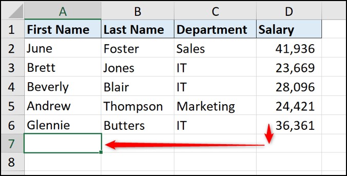
- In the first cell of an empty column, enter the desired result based on the data in the adjacent column. For example, if you want to extract the first name from a “Full Name” column, enter the first name in the first cell of the new column.
- In the next cell down, start typing the next first name. Flash Fill will recognize the pattern and suggest the rest of the names.
- Press “Enter” to accept the suggestions.
-
Combining Data:
- In the first cell of an empty column, enter the desired combination of data from the adjacent columns. For example, if you want to combine “First Name” and “Last Name” columns, enter the full name in the first cell of the new column.
- In the next cell down, start typing the next full name. Flash Fill will recognize the pattern and suggest the rest of the names.
- Press “Enter” to accept the suggestions.
-
Reformatting Data:
- In the first cell of an empty column, enter the desired reformatting of data from the adjacent column. For example, if you want to change phone number formatting, enter the reformatted phone number in the first cell of the new column.
- In the next cell down, start typing the next reformatted phone number. Flash Fill will recognize the pattern and suggest the rest of the phone numbers.
- Press “Enter” to accept the suggestions.
Alt Text: Example of using Flash Fill to extract first names from a list of full names in Excel.
Tip: Flash Fill works best when there is a clear and consistent pattern in your data. If Flash Fill doesn’t automatically recognize the pattern, try providing a few more examples. You can also manually trigger Flash Fill by going to the “Data” tab and clicking on “Flash Fill” in the “Data Tools” group, or by using the shortcut
Ctrl + E.
8. Conveying Insights Through Charts and Graphs
Visualizing data through charts and graphs makes it easier to understand and communicate complex information. Excel offers a variety of chart types to suit different data sets and purposes.
-
Creating a Basic Chart:
- Select the data you want to include in the chart.
- Go to the “Insert” tab on the ribbon and click on the chart type you want to create (e.g., “Column,” “Line,” “Pie,” “Bar,” “Scatter”).
- Choose a chart subtype.
- Excel will automatically create the chart based on the selected data.
-
Customizing a Chart:
- Chart Elements: Add or remove chart elements such as titles, axis labels, legends, data labels, and gridlines. Click on the chart, then click the “+” icon next to the chart to add or remove elements.
- Chart Styles and Colors: Change the style and colors of the chart. Click on the chart, then click the “paintbrush” icon next to the chart to choose a style and color scheme.
- Chart Filters: Filter the data displayed in the chart. Click on the chart, then click the “funnel” icon next to the chart to filter the data.
- Chart Type: Change the type of chart. Click on the chart, go to the “Chart Design” tab on the ribbon, and click on “Change Chart Type.”
-
Choosing the Right Chart Type:
- Column Chart: Use column charts to compare values across different categories.
- Line Chart: Use line charts to show trends over time.
- Pie Chart: Use pie charts to show the proportion of each category to the whole.
- Bar Chart: Use bar charts to compare values across different categories when the category names are long.
- Scatter Chart: Use scatter charts to show the relationship between two sets of data.
Alt Text: Demonstrating the process of creating a chart in Excel by selecting data and choosing a chart type.
Tip: Keep your charts simple and easy to understand. Use clear and concise titles and labels. Choose the chart type that best represents your data and communicates your message. Regularly update your charts as your data changes.
9. Summarizing Data Effectively with PivotTables
PivotTables are a powerful tool in Excel for summarizing and analyzing large datasets. They allow you to quickly extract meaningful insights by reorganizing and summarizing data in different ways.
-
Creating a PivotTable:
- Select the data you want to include in the PivotTable.
- Go to the “Insert” tab on the ribbon and click on “PivotTable.”
- In the Create PivotTable dialog box, confirm the data range and choose where to place the PivotTable (new worksheet or existing worksheet).
- Click “OK.”
- The PivotTable Fields pane will appear, allowing you to drag and drop fields into the “Rows,” “Columns,” “Values,” and “Filters” areas.
-
Customizing a PivotTable:
- Rows and Columns: Drag fields into the “Rows” and “Columns” areas to group and categorize your data.
- Values: Drag fields into the “Values” area to perform calculations such as sum, count, average, min, and max.
- Filters: Drag fields into the “Filters” area to filter the data displayed in the PivotTable.
- Grouping: Group data by date, number, or text to create higher-level summaries.
- Sorting: Sort data by row or column to arrange the data in a specific order.
- Calculated Fields: Create custom calculations based on the existing fields in the PivotTable.
Alt Text: Steps to create a PivotTable in Excel, highlighting the data selection and placement options.
Tip: Start by understanding the structure of your data and the questions you want to answer. Experiment with different arrangements of fields in the PivotTable to find the most meaningful insights. Use grouping and filtering to focus on specific subsets of data. Regularly refresh your PivotTables to ensure they reflect the latest data.
10. Protecting Worksheet Data to Maintain Accuracy
Protecting your worksheet data is essential to maintain its accuracy and integrity. Excel offers various protection options, including locking cells, protecting sheets, and protecting workbooks.
-
Locking Cells:
- Select the cells you want to lock.
- Right-click and choose “Format Cells.”
- Go to the “Protection” tab and check the “Locked” box.
- Click “OK.”
- To enable cell locking, you must protect the sheet (see below).
-
Protecting a Sheet:
- Go to the “Review” tab on the ribbon and click on “Protect Sheet.”
- Enter a password (optional) and choose the actions you want to allow users to perform (e.g., “Select locked cells,” “Select unlocked cells,” “Format cells,” “Insert rows,” “Delete columns”).
- Click “OK.”
- If you entered a password, you will be prompted to confirm it.
-
Protecting a Workbook:
- Go to the “File” tab and click on “Info.”
- Click on “Protect Workbook” and choose a protection option (e.g., “Mark as Final,” “Encrypt with Password,” “Protect Current Sheet,” “Protect Workbook Structure”).
- Follow the prompts to set up the protection.
Alt Text: Demonstrating the process of protecting a worksheet in Excel, including selecting allowed actions and setting a password.
Tip: Plan your protection strategy carefully to ensure that users can still perform necessary tasks while preventing accidental or malicious changes. Use passwords to protect sensitive data, but remember to keep the passwords in a safe place. Regularly review and update your protection settings as your data and user needs change.
11. Optimizing Data Handling with Power Query and Power Pivot
Power Query and Power Pivot are advanced tools in Excel that allow you to import, transform, and analyze large and complex datasets. Mastering these tools can significantly enhance your data handling capabilities.
-
Power Query:
- Importing Data: Use Power Query to import data from various sources, including Excel files, CSV files, databases, and web pages. Go to the “Data” tab on the ribbon and click on “Get Data” to choose a data source.
- Transforming Data: Use Power Query to clean and transform data by performing operations such as filtering, sorting, removing duplicates, splitting columns, and changing data types. The Power Query Editor provides a user-friendly interface for these operations.
- Loading Data: Load the transformed data into an Excel worksheet or the Power Pivot data model.
-
Power Pivot:
- Creating Data Models: Use Power Pivot to create data models by importing data from multiple tables and creating relationships between them. Go to the “Power Pivot” tab on the ribbon and click on “Manage” to open the Power Pivot window.
- Writing DAX Formulas: Use DAX (Data Analysis Expressions) formulas to perform calculations and analyses on the data in the data model. DAX is a powerful formula language that allows you to create custom measures and calculated columns.
- Analyzing Data: Use PivotTables and PivotCharts to analyze the data in the data model and gain insights.
Alt Text: Interface of Power Query Editor, showcasing data transformation and cleaning operations.
Tip: Start by understanding the structure and quality of your data. Use Power Query to clean and transform the data before loading it into Power Pivot. Learn the basics of DAX and practice writing formulas to perform common calculations. Use Power Pivot to create data models that reflect the relationships between your data.
12. Automating Repetitive Tasks with Macros and VBA
Macros and VBA (Visual Basic for Applications) allow you to automate repetitive tasks in Excel, saving time and reducing errors. Mastering these tools can significantly enhance your productivity.
-
Recording a Macro:
- Go to the “View” tab on the ribbon and click on “Macros.”
- Choose “Record Macro.”
- Enter a macro name, assign a shortcut key (optional), and choose where to store the macro (this workbook or personal macro workbook).
- Click “OK.”
- Perform the tasks you want to automate.
- Click on “Stop Recording” in the “View” tab.
-
Running a Macro:
- Go to the “View” tab on the ribbon and click on “Macros.”
- Choose “View Macros.”
- Select the macro you want to run and click “Run.”
- Alternatively, use the assigned shortcut key to run the macro.
-
Editing a Macro with VBA:
- Go to the “View” tab on the ribbon and click on “Macros.”
- Choose “View Macros.”
- Select the macro you want to edit and click “Edit.”
- The VBA editor will open, allowing you to view and edit the VBA code.
Tip: Start by recording simple macros to automate basic tasks. Learn the basics of VBA and practice writing code to customize your macros. Use comments to document your code and make it easier to understand. Regularly test your macros to ensure they are working correctly. LEARNS.EDU.VN provides courses on VBA to extend your knowledge.
Frequently Asked Questions (FAQ)
1. How long does it take to learn Excel at home?
The time it takes to learn Excel varies depending on your goals and the depth of knowledge you need. Basic proficiency can be achieved in a few weeks with consistent effort, while mastering advanced features may take several months. LEARNS.EDU.VN offers structured learning paths to guide you.
2. What are the best resources for learning Excel at home?
There are numerous resources available, including online courses, tutorials, books, and practice exercises. Websites like LEARNS.EDU.VN provide comprehensive materials tailored to different skill levels.
3. Is it possible to learn Excel for free?
Yes, many free resources are available, such as YouTube tutorials, blog posts, and community forums. However, structured courses often provide a more efficient and comprehensive learning experience.
4. What are the key Excel skills to focus on for data analysis?
Key skills include formulas, functions (e.g., VLOOKUP, SUMIF, COUNTIF), PivotTables, charts, and data validation. These skills enable you to analyze, summarize, and visualize data effectively.
5. How can I practice Excel skills at home?
Practice by working on real-world projects, such as budgeting, tracking expenses, or analyzing sales data. Experiment with different features and functions, and don’t be afraid to make mistakes.
6. What are some common mistakes to avoid when learning Excel?
Common mistakes include using absolute references incorrectly, not understanding formula syntax, and neglecting data validation. Always double-check your formulas and data to ensure accuracy.
7. How important is Excel for career advancement?
Excel is a highly valued skill in many industries, including finance, accounting, marketing, and operations. Proficiency in Excel can significantly enhance your career prospects and earning potential.
8. Can I use Excel on a Mac?
Yes, Microsoft Excel is available for both Windows and Mac operating systems. The features and functionalities are largely the same across both platforms.
9. What is the difference between Excel and Google Sheets?
Excel is a desktop application with a wide range of features and capabilities, while Google Sheets is a web-based spreadsheet program that offers real-time collaboration and accessibility from any device with an internet connection. Both tools have their strengths and weaknesses.
10. How can I stay updated with the latest Excel features and updates?
Follow Microsoft’s official Excel blog, join online communities and forums, and subscribe to newsletters from reputable sources like LEARNS.EDU.VN.
Enhance Your Excel Skills with LEARNS.EDU.VN
Ready to take your Excel skills to the next level? LEARNS.EDU.VN offers a wide range of courses and resources tailored to your needs. Whether you’re a beginner or an experienced user, we have the tools and expertise to help you succeed.
- Comprehensive Courses: Our structured courses cover everything from the basics to advanced techniques.
- Expert Instructors: Learn from experienced professionals who are passionate about Excel.
- Practical Exercises: Practice your skills with real-world projects and exercises.
- Community Support: Connect with other learners and share your knowledge.
Visit LEARNS.EDU.VN today to explore our offerings and start your journey toward Excel mastery. Contact us at 123 Education Way, Learnville, CA 90210, United States, or WhatsApp +1 555-555-1212.
Embrace the opportunity to transform your Excel skills at home with learns.edu.vn. Unlock new possibilities, enhance your career, and become an Excel expert today.