Principal Component Analysis (PCA) is a powerful technique extensively applied in machine learning. This article from LEARNS.EDU.VN provides a step-by-step guide on how PCA works, covering its definition, applications, and benefits. Discover how to simplify complex datasets while retaining crucial information. Explore dimensionality reduction, variance explanation, and feature extraction techniques.
1. Understanding Principal Component Analysis (PCA)
Principal Component Analysis (PCA) is a dimensionality reduction technique used in machine learning to transform a large set of variables into a smaller one that still contains most of the information in the large set. This reduction simplifies data analysis and visualization. According to a study by the University of Washington, PCA can significantly improve the efficiency of machine learning algorithms by reducing the number of features they need to process.
1.1. What is Dimensionality Reduction?
Dimensionality reduction is the process of reducing the number of variables (or dimensions) in a dataset while retaining its essential information. It is a crucial step in machine learning to simplify models and improve their performance. Fewer dimensions mean less computational complexity and faster training times.
1.2. Benefits of PCA
PCA offers several advantages in machine learning:
- Simplified Data: Reduces the number of variables, making the dataset easier to understand and visualize.
- Improved Model Performance: Eliminates noise and irrelevant features, which can improve the accuracy and efficiency of machine learning models.
- Faster Training Times: Reduces the computational complexity, leading to faster model training.
- Overfitting Prevention: Helps prevent overfitting by reducing the number of parameters the model needs to learn.
- Feature Extraction: Creates new, uncorrelated variables (principal components) that capture the most important information in the data.
1.3. PCA vs. Other Dimensionality Reduction Techniques
While PCA is a popular choice, other dimensionality reduction techniques exist. Here’s a comparison:
| Technique | Description | Advantages | Disadvantages |
|---|---|---|---|
| Principal Component Analysis (PCA) | Transforms data into uncorrelated principal components, ordered by variance. | Simple, fast, effective for linear data. | Assumes linearity, can be sensitive to outliers. |
| Linear Discriminant Analysis (LDA) | Maximizes the separability between classes. | Effective for classification tasks, handles multiple classes. | Assumes data is normally distributed, sensitive to outliers. |
| t-Distributed Stochastic Neighbor Embedding (t-SNE) | Reduces dimensionality while preserving local structure. | Excellent for visualizing high-dimensional data, captures non-linear relationships. | Computationally expensive, sensitive to parameter tuning, can distort global structure. |
| Autoencoders | Neural networks that learn to encode and decode data. | Can capture complex, non-linear relationships, can be used for feature extraction and anomaly detection. | Requires significant training data and computational resources, can be difficult to interpret the learned features. |
2. Core Concepts of PCA
To fully grasp how PCA works, it’s essential to understand the following core concepts:
2.1. Variance
Variance measures how spread out the data points are from the mean. In PCA, the goal is to find the directions (principal components) that maximize the variance. Higher variance indicates that the data is more spread out along that direction, meaning it contains more information.
2.2. Covariance
Covariance measures how two variables change together. A positive covariance means that the variables tend to increase or decrease together, while a negative covariance means that one variable increases as the other decreases. PCA uses the covariance matrix to understand the relationships between the variables in the dataset.
2.3. Eigenvectors and Eigenvalues
Eigenvectors and eigenvalues are mathematical concepts used to determine the principal components of the data. Eigenvectors represent the directions of the principal components, while eigenvalues represent the amount of variance explained by each principal component. A higher eigenvalue indicates that the corresponding eigenvector captures more variance in the data. According to research from MIT, these values are critical for identifying the most important axes of variation in the data.
2.4. Principal Components
Principal components are new variables created as linear combinations of the original variables. These components are uncorrelated and ordered by the amount of variance they explain. The first principal component explains the most variance, the second explains the second most, and so on.
3. Step-by-Step Guide to Performing PCA
PCA can be broken down into five main steps. Below, we’ll explain each step in detail.
3.1. Step 1: Data Standardization
The first step in PCA is to standardize the data. Standardization involves scaling the variables so that they have a mean of 0 and a standard deviation of 1. This ensures that each variable contributes equally to the analysis, regardless of its original scale. Without standardization, variables with larger ranges can dominate the results.
3.1.1. Why Standardize?
Standardization is critical because PCA is sensitive to the variances of the initial variables. If the variables have significantly different ranges, those with larger ranges will dominate, leading to biased results.
3.1.2. How to Standardize
To standardize a variable, subtract the mean and divide by the standard deviation:
z = (x - μ) / σWhere:
zis the standardized valuexis the original valueμis the mean of the variableσis the standard deviation of the variable
3.1.3. Example of Standardization
Let’s say we have two variables, A and B, with the following values:
- Variable A: [10, 20, 30, 40, 50]
- Variable B: [1, 2, 3, 4, 5]
First, calculate the mean and standard deviation for each variable:
- Variable A: Mean = 30, Standard Deviation = 15.81
- Variable B: Mean = 3, Standard Deviation = 1.58
Now, standardize each value:
- Standardized A: [-1.26, -0.63, 0, 0.63, 1.26]
- Standardized B: [-1.26, -0.63, 0, 0.63, 1.26]
After standardization, both variables have the same scale, ensuring they contribute equally to the PCA.
3.2. Step 2: Covariance Matrix Computation
The next step is to compute the covariance matrix of the standardized data. The covariance matrix shows how the variables vary together. This matrix is symmetric, with the variances of the variables on the main diagonal and the covariances between pairs of variables off the diagonal.
3.2.1. What is the Covariance Matrix?
The covariance matrix is a square matrix where each element represents the covariance between two variables. For a dataset with p variables, the covariance matrix is a p × p matrix.
3.2.2. How to Compute the Covariance Matrix
The covariance between two variables X and Y is calculated as:
Cov(X, Y) = Σ [(Xi - μX) * (Yi - μY)] / (n - 1)Where:
XiandYiare the individual values of the variablesμXandμYare the means of the variablesnis the number of data points
3.2.3. Interpreting the Covariance Matrix
The covariance matrix provides insights into the relationships between variables:
- Positive Covariance: Indicates that the variables tend to increase or decrease together.
- Negative Covariance: Indicates that one variable increases as the other decreases.
- Zero Covariance: Indicates that the variables are uncorrelated.
3.2.4. Example of Covariance Matrix Computation
Consider a dataset with two variables, X and Y:
| Data Point | X | Y |
|---|---|---|
| 1 | 1 | 2 |
| 2 | 2 | 4 |
| 3 | 3 | 6 |
| 4 | 4 | 8 |
| 5 | 5 | 10 |
First, calculate the means:
- μX = (1 + 2 + 3 + 4 + 5) / 5 = 3
- μY = (2 + 4 + 6 + 8 + 10) / 5 = 6
Next, compute the covariance matrix:
Cov(X, X) = Σ [(Xi - μX) * (Xi - μX)] / (n - 1) = 2.5
Cov(Y, Y) = Σ [(Yi - μY) * (Yi - μY)] / (n - 1) = 10
Cov(X, Y) = Σ [(Xi - μX) * (Yi - μY)] / (n - 1) = 5
Cov(Y, X) = Σ [(Yi - μY) * (Xi - μX)] / (n - 1) = 5
The covariance matrix is:
| 2.5  5  |
| 5   10 |
3.3. Step 3: Eigenvalue and Eigenvector Calculation
This step involves computing the eigenvectors and eigenvalues of the covariance matrix. Eigenvectors represent the directions of the principal components, while eigenvalues represent the amount of variance explained by each principal component.
3.3.1. What are Eigenvectors and Eigenvalues?
- Eigenvectors: Vectors that do not change direction when a linear transformation is applied. In PCA, they represent the directions of the principal components.
- Eigenvalues: Scalars that indicate the amount of variance explained by each eigenvector. Larger eigenvalues correspond to eigenvectors that capture more variance.
3.3.2. How to Calculate Eigenvectors and Eigenvalues
For a covariance matrix A, the eigenvectors v and eigenvalues λ satisfy the equation:
Av = λvSolving this equation involves finding the values of λ (eigenvalues) that satisfy the characteristic equation:
det(A - λI) = 0Where I is the identity matrix. Once the eigenvalues are found, the corresponding eigenvectors can be calculated by solving the equation (A – λI)v = 0.
3.3.3. Example of Eigenvalue and Eigenvector Calculation
Using the covariance matrix from the previous example:
| 2.5  5  |
| 5   10 |
The characteristic equation is:
det(A - λI) = (2.5 - λ)(10 - λ) - 5*5 = 0Solving for λ:
λ^2 - 12.5λ - 25 + 25 = 0
λ^2 - 12.5λ = 0
λ(λ - 12.5) = 0
λ1 = 0
λ2 = 12.5
The eigenvalues are λ1 = 0 and λ2 = 12.5.
Now, calculate the eigenvectors:
For λ1 = 0:
(A - λ1I)v = 0
| 2.5  5  | | v1 | = | 0 |
| 5   10 | | v2 | = | 0 |
Solving this system of equations gives the eigenvector v1 = [-2, 1].
For λ2 = 12.5:
(A - λ2I)v = 0
| -10  5  | | v1 | = | 0 |
| 5  -2.5 | | v2 | = | 0 |
Solving this system of equations gives the eigenvector v2 = [0.5, 1].
3.4. Step 4: Feature Vector Creation
In this step, you create a feature vector by selecting the eigenvectors that correspond to the largest eigenvalues. The feature vector is a matrix whose columns are the eigenvectors you want to keep. This is where dimensionality reduction happens.
3.4.1. What is a Feature Vector?
A feature vector is a matrix that contains the eigenvectors of the principal components you want to retain. The number of columns in the feature vector determines the number of dimensions in the reduced dataset.
3.4.2. How to Create a Feature Vector
- Sort Eigenvalues: Sort the eigenvalues in descending order.
- Select Eigenvectors: Choose the eigenvectors that correspond to the largest eigenvalues. The number of eigenvectors you select determines the number of dimensions in the reduced dataset.
- Create Matrix: Form a matrix with the selected eigenvectors as columns. This matrix is the feature vector.
3.4.3. Example of Feature Vector Creation
From the previous example, we have the following eigenvalues and eigenvectors:
- λ1 = 0, v1 = [-2, 1]
- λ2 = 12.5, v2 = [0.5, 1]
Since λ2 is larger than λ1, we select v2 as the first principal component. If we want to reduce the dataset to one dimension, the feature vector will be:
| 0.5 |
| 1   |
3.5. Step 5: Data Recasting
The final step is to recast the original data along the axes of the principal components. This involves multiplying the transpose of the original data by the transpose of the feature vector.
3.5.1. Why Recast Data?
Recasting the data transforms it into a new coordinate system defined by the principal components. This allows you to represent the data in a lower-dimensional space while retaining as much of the original variance as possible.
3.5.2. How to Recast Data
To recast the data, perform the following matrix multiplication:
FinalData = OriginalData * FeatureVectorWhere:
OriginalDatais the standardized original dataFeatureVectoris the feature vector created in the previous stepFinalDatais the reduced-dimensional data
3.5.3. Example of Data Recasting
Let’s assume our original data (after standardization) is:
| 1  2 |
| 2  4 |
| 3  6 |
| 4  8 |
| 5  10 |
And our feature vector is:
| 0.5 |
| 1   |
Then, the recasted data is:
| 1*0.5 + 2*1   | = | 2.5  |
| 2*0.5 + 4*1   | = | 5    |
| 3*0.5 + 6*1   | = | 7.5  |
| 4*0.5 + 8*1   | = | 10   |
| 5*0.5 + 10*1  | = | 12.5 |
The final data is now represented in one dimension, capturing the most significant variance in the original data.
4. Practical Applications of PCA in Machine Learning
PCA is used in many different applications. Here are some examples:
4.1. Image Compression
PCA can reduce the size of image files by reducing the number of dimensions needed to represent the image. Each image can be represented with fewer components without losing essential image qualities.
4.2. Facial Recognition
PCA is used to extract relevant features from facial images, which can then be used for identification. By reducing the dimensionality of the image data, PCA makes it easier to compare and classify faces.
4.3. Gene Expression Analysis
In genomics, PCA can be used to identify patterns in gene expression data. This can help researchers understand how genes are regulated and how they contribute to different diseases.
4.4. Stock Market Analysis
PCA can be used to identify the most important factors that influence stock prices. This can help investors make better decisions about which stocks to buy and sell.
5. Advanced Techniques and Considerations
While the basic PCA process is straightforward, several advanced techniques and considerations can further enhance its effectiveness.
5.1. Kernel PCA
Kernel PCA extends the capabilities of standard PCA by using kernel functions to perform non-linear dimensionality reduction. This technique is particularly useful when dealing with data that has complex, non-linear relationships.
5.2. Incremental PCA
Incremental PCA is designed for large datasets that cannot fit into memory. It processes the data in batches, updating the principal components incrementally. This approach allows you to perform PCA on datasets that would otherwise be too large to handle.
5.3. Sparse PCA
Sparse PCA aims to find principal components that are sparse, meaning they have few non-zero elements. This can improve the interpretability of the components and reduce the risk of overfitting.
5.4. Choosing the Number of Components
Selecting the right number of components is a critical decision in PCA. Keeping too many components can retain noise and irrelevant information, while keeping too few can lose essential details.
5.4.1. Explained Variance Ratio
The explained variance ratio is the proportion of the dataset’s variance that each principal component captures. You can use this to decide how many components to keep. Typically, you’d want to keep enough components to explain a high percentage of the variance (e.g., 95%).
5.4.2. Scree Plot
A scree plot is a line plot that shows the eigenvalues of the principal components in descending order. The “elbow” of the plot (where the line starts to flatten out) can indicate the optimal number of components to retain.
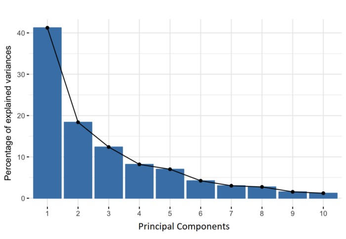 Percentage of Variance (Information) for each by PC
6. Common Pitfalls and How to Avoid Them
While PCA is a powerful technique, it’s essential to be aware of common pitfalls and how to avoid them.
6.1. Data Scaling Issues
Failing to standardize the data can lead to biased results. Always ensure that your data is properly scaled before performing PCA.
6.2. Linearity Assumption
PCA assumes that the data is linearly related. If your data has strong non-linear relationships, consider using Kernel PCA or other non-linear dimensionality reduction techniques.
6.3. Outlier Sensitivity
PCA can be sensitive to outliers. Consider removing or transforming outliers before applying PCA.
6.4. Over-Interpretation of Components
Be cautious when interpreting the principal components. They are linear combinations of the original variables and may not have a clear, intuitive meaning.
7. Examples of PCA Implementation
Here are examples of how PCA is implemented in different fields.
7.1. In Finance
Financial analysts use PCA to identify key factors driving stock returns. By reducing the number of variables, they can create more manageable and interpretable models.
7.2. In Healthcare
Researchers use PCA to analyze patient data and identify patterns that can help diagnose diseases. This can lead to earlier and more accurate diagnoses, improving patient outcomes.
7.3. In Environmental Science
Environmental scientists use PCA to analyze environmental data and identify the most important factors contributing to pollution. This can help policymakers develop more effective strategies for reducing pollution.
8. Educational Resources for PCA
Several educational resources can help you learn more about PCA.
8.1. Online Courses
Sites like Coursera, Udacity, and edX offer courses on machine learning that cover PCA. These courses provide a structured learning experience with video lectures, assignments, and projects.
8.2. Books
Several books provide in-depth coverage of PCA, including “The Elements of Statistical Learning” by Hastie, Tibshirani, and Friedman, and “Pattern Recognition and Machine Learning” by Christopher Bishop.
8.3. Tutorials
Websites like LEARNS.EDU.VN offer tutorials and articles on PCA. These resources provide practical guidance and examples to help you understand and apply PCA.
9. The Future of PCA
PCA remains a fundamental technique in machine learning, but its future is evolving with advances in technology.
9.1. Integration with Deep Learning
PCA is increasingly being used as a preprocessing step for deep learning models. By reducing the dimensionality of the input data, PCA can improve the efficiency and performance of deep learning algorithms.
9.2. Automated PCA
Automated machine learning (AutoML) platforms are making it easier to apply PCA. These platforms automate the process of selecting the optimal number of components and tuning other PCA parameters.
9.3. Real-Time PCA
With the growth of real-time data processing, PCA is being adapted for real-time applications. This involves developing algorithms that can perform PCA on streaming data, enabling real-time dimensionality reduction and feature extraction.
10. FAQ About PCA
Here are some frequently asked questions about PCA:
10.1. What does PCA plot tell you?
A PCA plot shows the relationships between samples in a dataset. Each point on the plot represents a sample, and the position of the point is determined by its principal component scores. Samples that are close together on the plot are more similar to each other than samples that are far apart.
10.2. Why is PCA used in machine learning?
PCA reduces the number of variables in a dataset while retaining the most important information. This can improve the efficiency and performance of machine learning models.
10.3. What is the main goal of PCA?
The main goal of PCA is to reduce the dimensionality of a dataset while retaining as much of the original variance as possible.
10.4. How do you interpret PCA results?
PCA results can be interpreted by examining the eigenvalues and eigenvectors. The eigenvalues indicate the amount of variance explained by each principal component, while the eigenvectors indicate the direction of each principal component.
10.5. What are the assumptions of PCA?
PCA assumes that the data is linearly related and that the variables have a multivariate normal distribution.
10.6. Can PCA be used for non-linear data?
Yes, Kernel PCA can be used for non-linear data. Kernel PCA uses kernel functions to perform non-linear dimensionality reduction.
10.7. How do you choose the number of principal components?
The number of principal components can be chosen by examining the explained variance ratio or by using a scree plot.
10.8. What is the difference between PCA and factor analysis?
PCA and factor analysis are both dimensionality reduction techniques, but they have different goals. PCA aims to reduce the number of variables in a dataset, while factor analysis aims to identify underlying factors that explain the correlations between variables.
10.9. How does PCA handle missing data?
PCA cannot handle missing data directly. Missing values must be imputed before applying PCA.
10.10. What is the role of standardization in PCA?
Standardization ensures that each variable contributes equally to the analysis, regardless of its original scale. This is important because PCA is sensitive to the variances of the initial variables.
Conclusion
PCA is a powerful tool for dimensionality reduction in machine learning. By following the steps outlined in this article, you can effectively apply PCA to simplify your datasets and improve the performance of your models. LEARNS.EDU.VN offers many more resources to help you master PCA and other machine learning techniques.
Ready to dive deeper into the world of data science and machine learning? Visit LEARNS.EDU.VN for more comprehensive guides, tutorials, and courses. Whether you’re looking to master PCA or explore other advanced techniques, LEARNS.EDU.VN provides the resources you need to succeed.
Contact Information:
- Address: 123 Education Way, Learnville, CA 90210, United States
- WhatsApp: +1 555-555-1212
- Website: LEARNS.EDU.VN
This article equips you with the knowledge to tackle dimensionality reduction confidently and efficiently. Discover how PCA can transform your approach to machine learning at learns.edu.vn.