A Survey On Deep Semi-supervised Learning explores algorithms that optimize objective functions with labeled and unlabeled samples, which can be found at LEARNS.EDU.VN. This article delves into maximum-margin methods, perturbation techniques, manifold-based approaches, and generative models, providing a comprehensive exploration of deep semi-supervised learning. Join us to discover everything you need to know about the foundations and applications of semi-supervised learning, deep neural networks, and machine learning strategies.
1. Understanding Deep Semi-Supervised Learning Surveys
Deep semi-supervised learning surveys focus on inductive learning algorithms designed to optimize objective functions directly using both labeled and unlabeled data. These methods, often termed “intrinsically semi-supervised,” bypass intermediate steps or supervised base learners. Instead, they commonly extend existing supervised techniques to incorporate unlabeled samples directly into the objective function.
1.1. Core Principles of Intrinsically Semi-Supervised Methods
Intrinsically semi-supervised methods rely on semi-supervised learning assumptions either explicitly or implicitly. For instance, maximum-margin methods leverage the low-density assumption, while most semi-supervised neural networks depend on the smoothness assumption. The primary techniques include:
- Maximum-Margin Methods: These methods aim to maximize the distance between data points and decision boundaries.
- Perturbation-Based Methods: Incorporate the smoothness assumption by applying perturbations to data points.
- Manifold-Based Techniques: Approximate the manifolds on which data lie.
- Generative Models: Use generative models to leverage unlabeled data effectively.
 Maximum Margin Classifier
1.2. The Role of Maximum-Margin Methods in Semi-Supervised Learning
Maximum-margin classifiers attempt to maximize the distance between given data points and the decision boundary. This corresponds to the semi-supervised low-density assumption. According to research highlighted at LEARNS.EDU.VN, when the margin between all data points and the decision boundary is large, the decision boundary is likely in a low-density area (Ben-David et al., 2009).
2. Detailed Look at Maximum-Margin Methods
Maximum-margin methods are vital in semi-supervised learning, focusing on maximizing the separation between data points and decision boundaries.
2.1. Support Vector Machines (SVM)
Support Vector Machines (SVM) are prominent maximum-margin classifiers. SVM is a classification method that maximizes the distance from the decision boundary to the closest data points while classifying data points correctly. SVMs are among the first maximum-margin approaches proposed for semi-supervised settings and have been extensively studied.
2.1.1. Objective of Support Vector Machines
The goal is to find a decision boundary that maximizes the margin, defined as the distance between the decision boundary and the nearest data points. A soft-margin SVM allows data points to violate the margin at a cost and supports mapping objects to higher-dimensional feature spaces using the kernel trick, as detailed by Bishop (2006).
2.1.2. Mathematical Formulation of SVMs
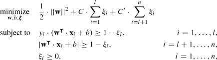
When training an SVM, the objective is to find a weight vector (mathbf {w} in mathbb {R}^d) with minimal magnitude and a bias variable (b in mathbb {R}), such that (y_i cdot (mathbf {w}^{intercal } cdot mathbf {x}_i + b) ge 1 – xi _i) for all data points (mathbf {x}_i in X_L). Here, (xi _i ge 0) is called the “slack variable” for (x_i), which allows (x_i) to violate the margin at some cost, incorporated into the objective function.
The optimization problem can be formulated as follows:
$$begin{aligned} begin{aligned}&underset{mathbf {w}, b, {varvec{xi }}}{text {minimize}}&frac{1}{2} cdot ||mathbf {w}||^2 + C cdot sum _{i=1}^l xi _i \&text {subject to}&y_i cdot (mathbf {w}^{intercal } cdot mathbf {x}_i + b) ge 1 – xi _i, ;&i = 1, ldots , l,\&&xi ge 0, ;&i = 1, ldots , l, end{aligned} end{aligned}$$
2.1.3. Role of the Constant Scaling Factor (C)
In the formulation above, (C in mathbb {R}) is a constant scaling factor for penalizing data points that violate the margin. When C is large, the optimal margin is narrow. When C is small, the optimal margin is wide. The constant C acts as a regularization parameter, governing the trade-off between the complexity of the decision boundary and prediction accuracy on the training set.
2.2. Semi-Supervised Support Vector Machines (S3VMs)
Semi-Supervised Support Vector Machines (S3VMs) extend the SVM concept. In addition to maximizing the margin and correctly classifying the labeled data, S3VMs aim to minimize the number of unlabeled data points violating the margin. Since the labels of the unlabeled data points are unknown, those violating the margin are penalized based on their distance to the closest margin boundary.
2.2.1. Optimization Problem for S3VMs
The intuitive extension of the optimization problem for S3VMs thus becomes:
Where (C’ in mathbb {R}) is the margin violation cost associated with unlabeled data points.
2.2.2. Challenges in Training S3VMs
A significant disadvantage of extending SVMs to the semi-supervised setting is that the optimization problem encountered when training S3VMs becomes non-convex and NP-hard. Therefore, efforts in S3VM research focus on training them efficiently.
2.2.3. Approaches to Solving S3VMs
Several approaches have been developed to address the challenges in training S3VMs, including:
- Mixed Integer Programming: Using the L1 norm instead of the L2 norm in the objective function.
- Iterative Label Assignment: Starting with a random label assignment and iteratively improving it.
- Convex Relaxations: Using semidefinite programming methods.
Chapelle et al. (2008) categorized S3VM optimization methods into combinatorial methods and continuous methods.
2.3. Continuous Methods for S3VMs
Continuous methods involve directly solving the optimization problem using label assignments (hat{y}_i = text {sign}(mathbf {w}^{intercal } cdot mathbf {x}_i + b)). These approaches are based on reformulating the problem as an optimization problem without constraints.
2.3.1. Reformulation of the Optimization Problem
The optimization problem can be reformulated as:
$$begin{aligned} begin{aligned} underset{mathbf {w}, b}{text {minimize}}&, , frac{1}{2} cdot ||mathbf {w}||^2 + C cdot sum _{i=1}^l text {max}left( 0, 1 – y_i cdot f(mathbf {x}_i)right) ~\&quad + C’ cdot sum _{i=l+1}^n text {max}left( 0, 1 – |f(mathbf {x}_i)|right) , end{aligned} end{aligned}$$
where (f(mathbf {x}_i) = mathbf {w}^{intercal } cdot mathbf {x}_i + b).
2.3.2. (nabla text {TSVM}) by Chapelle and Zien
This approach underlies (nabla text {TSVM}) by Chapelle and Zien (2005), which is based on a smooth approximation of the object function obtained by squaring the loss for the labeled data points and approximating the loss for the unlabeled data points with an exponential function.
2.4. Limitations of S3VMs
Like most semi-supervised learning methods, S3VMs are not guaranteed to perform better than their supervised counterparts (Singh et al., 2009). Performance can degrade if the underlying assumptions are violated.
2.5. Mitigating Performance Degradation in S3VMs
Li and Zhou (2015) proposed mitigating performance degradation by considering a diverse set of low-density separators and choosing the separator that performs best under the worst possible ground truth.
2.5.1. The S4VM Algorithm
The S4VM (safe S3VM) algorithm consists of two stages:
- Constructing a diverse set of low-density decision boundaries.
- Choosing the decision boundary with maximal worst-case performance gain over the supervised decision boundary.
2.5.2. Mathematical Formulation of Performance Gain
The performance gain is formulated as the resulting increase in the number of correctly labeled data points minus the increase in the number of incorrectly labeled data. The latter term is multiplied by a factor (lambda in mathbb {R}), governing the amount of risk of performance degradation one wishes to take. Formally, this is captured by a scoring function (J(hat{mathbf {y}}, mathbf {y}, mathbf {y}^text {svm})) for a set of predicted labels (hat{mathbf {y}}), ground truth (mathbf {y}), and supervised SVM predictions (mathbf {y}^text {svm}) defined as:
$$begin{aligned} J(hat{mathbf {y}}, mathbf {y}, mathbf {y}^text {svm}) = gain(hat{mathbf {y}}, mathbf {y}, mathbf {y}^text {svm}) – lambda cdot lose(hat{mathbf {y}}, mathbf {y}, mathbf {y}^text {svm}), end{aligned}$$
2.5.3. The Optimal Label Assignment
The optimal label assignment (bar{mathbf {y}}) in the worst-case true labeling can then be found as:
$$begin{aligned} bar{mathbf {y}} in ,mathop {{{,mathrm{arg,max},}}}limits _{mathbf {y} in {pm 1}^u} left[ min _{hat{mathbf {y}} in mathcal {M}} J(mathbf {y}, hat{mathbf {y}}, mathbf {y}^text {svm}) right] , end{aligned}$$
Li and Zhou (2015) proposed a convex relaxation of the problem to effectively find a good candidate solution.
2.6. Gaussian Processes in Semi-Supervised Learning
Lawrence and Jordan (2005) extended Gaussian processes to handle unlabeled data, providing another approach to margin maximization.
2.6.1. Gaussian Processes Overview
Gaussian processes are non-parametric models that estimate the posterior probability over the function f mapping points in the input space to a continuous output space.
2.6.2. Extension to Semi-Supervised Learning
Lawrence and Jordan (2005) extended Gaussian processes for binary classification to the semi-supervised case by incorporating the unlabeled data points into the likelihood function.
2.6.3. Likelihood for Unlabeled Data
The likelihood for an unlabeled data point (mathbf {x}) is low when it is close to the decision boundary (i.e., when (f(mathbf {x})) is close to 0) and high when it is far away from the decision boundary.
2.6.4. Impact on Posterior Variance
Contrary to supervised Gaussian processes, introducing additional unlabeled data can increase the posterior variance, which stems from the observation that the likelihood function for a single unlabeled data point (mathbf {x}^*) can be bimodal if (f(mathbf {x}^*)) is close to 0.
2.7. Density Regularization
Another way to encourage the decision boundary to pass through a low-density area is to explicitly incorporate the amount of overlap between the estimated posterior class probabilities into the cost function.
2.7.1. Maximum A Posteriori (MAP) Framework
Grandvalet and Bengio (2005) proposed formalizing this in the maximum a posteriori (MAP) framework by imposing a prior on the model parameters, favoring parameters inducing small class overlap in the predictive model.
2.7.2. Incorporation of p(x) into the Objective Function
Corduneanu and Jaakkola (2003) proposed to directly incorporate an estimate of p(x), the distribution over the input data, into the objective function.
2.7.3. Density Prior in Decision Trees
Liu et al. (2013, 2015) proposed to incorporate the prior density into the node-splitting criterion of decision trees.
2.8. Pseudo-Labeling as Margin Maximization
Depending on the base learner used, the self-training approach can also be regarded as a margin-maximization method.
2.8.1. Self-Training with Supervised SVMs
When using self-training with supervised SVMs, the decision boundary is iteratively pushed away from the unlabeled samples, exploiting the low-density assumption.
3. Perturbation-Based Methods
Perturbation-based methods leverage the smoothness assumption, which states that a predictive model should be robust to local input perturbations.
3.1. Core Principle of Perturbation-Based Methods
The central idea is that when a data point is perturbed with noise, the predictions for the noisy and clean inputs should be similar.
3.2. Implementation Approaches
Two primary approaches exist for incorporating the smoothness assumption:
- Applying noise to the input data points and incorporating the difference between clean and noisy predictions into the loss function.
- Implicitly applying noise to the data points by perturbing the classifier itself.
3.3. Neural Networks in Perturbation-Based Methods
Perturbation-based methods are often implemented with neural networks because of their straightforward incorporation of additional (unsupervised) loss terms into their objective function.
3.4. Semi-Supervised Neural Networks
Semi-supervised neural networks differ from neural networks used for feature extraction. The unlabeled data is incorporated directly into the optimization objective rather than in a separate preprocessing step.
3.5. Short Introduction to Neural Networks
A neural network computes an output vector by propagating an input vector through a network of simple processing elements with weighted connections. Nodes are grouped into layers and contain an activation function that determines their output.
3.5.1. Supervised Neural Networks
In supervised neural networks, weights are optimized to calculate the desired output vector for a given input vector.
3.5.2. Loss Function
A loss function (ell ) calculates the cost associated with output layer activations (f(mathbf {x};W)) for a data point (mathbf {x}) with true label y.
3.5.3. Backpropagation
Weights are iteratively optimized by passing input samples through the network and propagating the share of one or more samples in the cost (mathcal {L}) backwards through the network via backpropagation.
3.6. Semi-Supervised Neural Networks
The simplicity and efficiency of the backpropagation algorithm for various loss functions make adding an unsupervised component to (mathcal {L}) attractive.
3.7. Ladder Networks
Ladder networks extend a feedforward network to incorporate unlabeled data by using the feedforward part of the network as the encoder of a denoising autoencoder, adding a decoder, and including a term in the cost function to penalize the reconstruction cost.
3.7.1. Structure of Ladder Networks
Ladder networks add an additional term to (mathcal {L}) to penalize the network’s sensitivity to input perturbations.
3.7.2. Denoising Autoencoder Component
The entire network is treated as the encoder part of a denoising autoencoder. Isotropic Gaussian noise is added to the input samples, and a decoder is added to reconstruct (mathbf {x}).
3.7.3. Reconstruction Cost
A reconstruction cost is added to the cost function of the network, penalizing the difference between the input data points and their reconstructions.
3.7.4. Differences from Regular Denoising Autoencoders
- Ladder networks inject noise at every layer, not just the first.
- Ladder networks utilize a different reconstruction cost calculation, penalizing local reconstructions of the hidden representations.
3.7.5. Final Semi-Supervised Cost Function
The final semi-supervised cost function of ladder networks becomes:
$$begin{aligned} mathcal {L}(W) = sum _{i = 1}^l ell (f(mathbf {x}_i), y_i) + sum _{i = 1}^n sum _{k = 1}^K text {ReconsCost}(mathbf {z}_i^{k}, hat{mathbf {z}}_i^{k}), end{aligned}$$
3.8. (Gamma )-Model
The (Gamma )-model, a simpler variant, only includes the reconstruction cost for the last layer and provides substantial performance improvements over the corresponding fully-supervised model.
3.9. Pseudo-Ensembles
Pseudo-ensembles perturb the neural network model itself. Robustness is promoted by penalizing the difference between the activations of the perturbed network and those of the original network.
3.9.1. General Framework
An unperturbed parent model is perturbed to obtain one or more child models.
3.9.2. Semi-Supervised Cost Function
The semi-supervised cost function consists of a supervised part and an unsupervised part. The former captures the loss of a perturbed network for labeled input data, and the latter captures the consistency across perturbed networks for unlabeled data points.
3.9.3. Dropout
A prominent method of inducing noise is dropout, which randomly sets weights to zero in each training iteration.
3.10. (Pi )-Model
The (Pi )-model trains two perturbed neural network models and penalizes differences in the final-layer activations using squared loss, starting with a zero weight on the unsupervised term.
3.11. Temporal Ensembling
Temporal ensembling compares the activations of the neural network at each epoch to the activations of the network at previous epochs, smoothing the network output over multiple model perturbations.
3.12. Mean Teacher
The mean teacher approach considers moving averages over connection weights instead of network activations and imposes noise on the input data to increase robustness.
3.12.1. Model Terminology
The model with averaged weights is the teacher model, and the latest model with weights (W_t) is the student model.
3.13. Virtual Adversarial Training
Virtual adversarial training takes the perturbation direction into account, approximating the perturbation that yields the largest change in network output for each data point.
3.13.1. Adversarial Loss Function
The adversarial loss function for a sample (mathbf {x}) can be defined as:
$$begin{aligned} ell (mathbf {x}) = D(f(mathbf {x};hat{W}), f(mathbf {x} + {varvec{gamma }}^{adv};W)), end{aligned}$$
3.14. Semi-Supervised Mixup
Semi-supervised mixup applies larger perturbations to the input, formalizing this in the mixup method, where predictions for a linear combination of feature vectors should be a linear combination of their labels.
3.14.1. Interpolation
The network is trained on the linearly interpolated data point ((hat{mathbf {x}}, hat{mathbf {y}})), where:
$$begin{aligned} hat{mathbf {x}}&= lambda cdot mathbf {x} + (1 – lambda ) cdot mathbf {x}’,\ hat{mathbf {y}}&= lambda cdot mathbf {y} + (1 – lambda ) cdot mathbf {y}’. end{aligned}$$
3.14.2. Application to Unlabeled Samples
The interpolation used in mixup can be applied to unlabeled samples by interpolating the predicted labels rather than the true labels.
4. Manifold-Based Techniques
Manifold-based techniques rely on the manifold assumption, where data lies on lower-dimensional manifolds.
4.1. The Manifold Assumption
The manifold assumption states that:
- The input space is composed of multiple lower-dimensional manifolds.
- Data points on the same manifold have the same label.
4.2. Types of Manifold-Based Methods
Two primary types of manifold-based methods exist:
- Manifold regularization techniques, which define a graph and penalize prediction differences for points with small geodesic distance.
- Manifold approximation techniques, which explicitly estimate manifolds and optimize an objective function.
4.3. Manifold Regularization
Manifold regularization defines a graph over data points and penalizes differences in predictions for points with small geodesic distance.
4.3.1. Similarity Graph
A similarity graph connects data points close in the input space with an edge, using edge weights to express similarity.
4.3.2. General Optimization Problem
Belkin et al. (2005, 2006) formulated the following general optimization problem:
$$begin{aligned} underset{f in mathcal {H}_K}{text {minimize}} quad sum _{i=1}^l left[ ell (f(mathbf {x}_i), y_i) right] + gamma cdot ||f||_K^2, end{aligned}$$
4.3.3. Manifold Regularization Term
The manifold regularization term (||f||_I^2) is defined as:
$$begin{aligned} ||f||_I^2 = frac{1}{2} cdot sum _{i = 1}^n sum _{j = 1}^n W_{ij} cdot (f(mathbf {x}_i) – f(mathbf {x}_j))^2. end{aligned}$$
4.3.4. Final Optimization Problem
The final optimization problem, including the manifold regularization term, becomes:
$$begin{aligned} underset{f in mathcal {H}_K}{text {minimize}} quad frac{1}{l} cdot sum _{i=1}^l ell (f(mathbf {x}_i), y_i) + gamma cdot ||f||_K^2 + gamma _U cdot ||f||_I^2, end{aligned}$$
4.3.5. Laplacian Support Vector Machines (LapSVMs)
LapSVMs maximize the margin and consistency of predictions along estimated manifolds.
4.4. Graph Construction Methods
Graph construction methods involve connectivity criteria and edge weighting schemes, making performance highly dependent on hyperparameter settings.
4.5. Ensemble Manifold Regularization
Geng et al. (2012) attempted to overcome the hyperparameter dependence by selecting a set of candidate Laplacians and finding their optimal linear combination.
4.5.1. Linear Combination of Laplacians
The optimization problem is posed as finding the linear combination of Laplacians that minimizes the manifold regularization objective.
4.5.2. Manifold Regularization Term
Using exponential weights in the Laplacian, the manifold regularization term (||f||_I^2) then becomes:
$$begin{aligned} ||f||_I^2&= mathbf {f}^{intercal } cdot L cdot mathbf {f} \&= mathbf {f}^{intercal } cdot left( sum _{j=1}^m mu _j cdot L_jright) cdot mathbf {f} \&= sum _{j=1}^m mu _j cdot ||f||_{I(j)}^2, end{aligned}$$
4.6. Manifold Approximation
Manifold approximation involves explicitly approximating the manifold and using it in a classification task.
4.6.1. Contractive Autoencoders (CAEs)
Rifai et al. (2011a) developed an approach where manifolds are first estimated using contractive autoencoders (CAEs) and then used by a supervised training algorithm.
4.6.2. Loss Function
The loss function (mathcal {L}) utilized by contractive autoencoders is:
$$begin{aligned} mathcal {L} = sum _{i=1}^n ell (g(h(mathbf {x}_i)), y_i) + lambda cdot ||J||_F^2, end{aligned}$$
4.6.3. Estimating Tangent Plane
Using singular value decomposition, the tangent plane is estimated at each input point to approximate the actual manifolds.
4.6.4. Learning a Manifold as an Atlas
Pitelis et al. (2013, 2014) suggested approximating charts explicitly, associating each with an affine subspace, and generating kernels for SVM-based supervised learning.
5. Generative Models
Generative models aim to model the process that generated the data.
5.1. Overview of Generative Models
Generative models explicitly model the data-generating distributions and can be powerful with prior knowledge about p(x, y).
5.2. Mixture Models
Mixture models assume that the data p(x, y) is composed of a mixture of k distributions. Each component (j = 1, dots , k) has a weight (pi _j), mean vector ({varvec{mu }}_j), and covariance matrix ({varvec{Sigma }}_j).
5.2.1. Expectations Maximization
The most likely parameters can be inferred, for example, via expectation-maximization (Dempster et al., 1977).
5.2.2. Application of Mixture Models
In the case of Gaussian mixture models, (p(y_i = c) = pi _c).
5.2.3. Limitations of Mixture Models
- The mixture model should be identifiable.
- Mixture models hinge on the assumption that the assumed model is correct.
5.3. Generative Adversarial Networks (GANs)
Generative adversarial networks (GANs) simultaneously construct generative and discriminative learners.
5.3.1. GAN Components
- A generator G generates data points indistinguishable from real data.
- A discriminator D predicts whether a given data point is real or fake.
5.3.2. Optimization Problem
The optimization problem can be formulated as:
$$begin{aligned} underset{G}{text {min}} , underset{D}{text {max}} quad V(D,G) = mathbb {E}_{mathbf {x} sim p(mathbf {x})} [log D(mathbf {x})] + mathbb {E}_{mathbf {z} sim p(mathbf {z})} [log (1 – D(G(mathbf {z}))], end{aligned}$$
5.3.3. CatGAN
Springenberg (2015) extended the GAN discriminator to use (|mathcal {Y}|) outputs, including a cross-entropy cost term to penalize misclassifications of real data.
5.3.4. Semi-Supervised GANs
Salimans et al. (2016) extended GANs to the semi-supervised setting by using (|mathcal {Y}|+1) outputs, adapting the loss function to include the cross-entropy loss.
5.4. Variational Autoencoders (VAEs)
Variational autoencoders (VAEs) treat each data point (mathbf {x}) as generated from latent variables (mathbf {z}), constraining (p(mathbf {z})) to a simple distribution.
5.4.1. Training a VAE
An encoder determines the parameters of a distribution (p(mathbf {z}|mathbf {x})) based on a data point (mathbf {x}). Latent vectors (mathbf {z}) can then be sampled from this distribution and passed through the decoder.
5.4.2. Application for Semi-Supervised Learning
Kingma et al. (2014) propose a two-step model:
- Training a VAE on both labeled and unlabeled data to extract meaningful latent representations.
- Implementing a VAE in which the latent representation is augmented with the label vector (mathbf {y}_i), introducing a classification network to infer label predictions.
6. Real-World Applications and Future Directions
Deep semi-supervised learning has various real-world applications. Recent advancements in image recognition, natural language processing, and medical diagnostics are driven by the enhanced capabilities of deep semi-supervised learning.
6.1. Overcoming Data Scarcity
These methods have been shown to be particularly effective in scenarios where labeled data is scarce but unlabeled data is abundant, thereby reducing annotation costs and improving model robustness.
6.2. Enhancing Model Generalization
Additionally, deep semi-supervised learning contributes to enhancing model generalization and reliability, which is vital for deploying machine learning systems in dynamic and uncertain real-world environments.
6.3. Future Research
Future research directions may include developing more efficient and robust algorithms, exploring new applications, and addressing the theoretical challenges of semi-supervised learning.
6.4. Advancements in Neural Networks
Further exploration of neural networks, along with practical advice, can be found at LEARNS.EDU.VN.
7. Conclusion
A survey on deep semi-supervised learning reveals significant methods that leverage both labeled and unlabeled data to optimize model performance. Techniques such as maximum-margin methods, perturbation-based approaches, manifold-based techniques, and generative models provide diverse strategies for enhancing learning outcomes. Discover more at LEARNS.EDU.VN and broaden your understanding of educational advancements.
Are you facing challenges in finding reliable educational resources or methods to enhance your learning process? Visit LEARNS.EDU.VN for expert guidance and comprehensive resources tailored to your needs. Our platform offers detailed articles, proven learning techniques, and personalized learning paths to help you succeed. Connect with us today to transform your learning experience.
Contact Information:
- Address: 123 Education Way, Learnville, CA 90210, United States
- WhatsApp: +1 555-555-1212
- Website: LEARNS.EDU.VN
8. Frequently Asked Questions (FAQ)
8.1. What is deep semi-supervised learning?
Deep semi-supervised learning is a machine-learning approach that combines a small amount of labeled data with a large amount of unlabeled data during training. This method is particularly useful when obtaining labeled data is costly or time-consuming.
8.2. How does semi-supervised learning differ from supervised learning?
Supervised learning uses only labeled data to train a model, whereas semi-supervised learning uses a combination of labeled and unlabeled data. Semi-supervised learning can often achieve higher accuracy than supervised learning when labeled data is scarce.
8.3. What are the primary assumptions in semi-supervised learning?
The primary assumptions include the smoothness assumption (points close to each other are likely to have the same label), the cluster assumption (data forms distinct clusters), and the manifold assumption (data lies on a lower-dimensional manifold).
8.4. What are maximum-margin methods in semi-supervised learning?
Maximum-margin methods aim to maximize the distance between the decision boundary and the data points. Support Vector Machines (SVMs) and Semi-Supervised Support Vector Machines (S3VMs) are examples of such methods.
8.5. What are perturbation-based methods?
Perturbation-based methods incorporate the smoothness assumption by applying small changes (perturbations) to the input data or the model itself and ensuring that the model’s predictions remain consistent.
8.6. How do manifold-based techniques work?
Manifold-based techniques assume that the data lies on a lower-dimensional manifold. These methods aim to learn the structure of this manifold and use it to guide the classification process.
8.7. What are generative models in semi-supervised learning?
Generative models, such as Generative Adversarial Networks (GANs) and Variational Autoencoders (VAEs), model the underlying data distribution and use this model to generate new samples or classify existing ones.
8.8. What is the role of unlabeled data in semi-supervised learning?
Unlabeled data helps to better understand the underlying data structure and improve model generalization, especially when labeled data is limited.
8.9. What are some real-world applications of deep semi-supervised learning?
Real-world applications include image recognition, natural language processing, medical diagnostics, and other areas where labeled data is scarce but unlabeled data is abundant.
8.10. Where can I find more resources and courses on deep semi-supervised learning?
More resources and courses can be found at learns.edu.vn, where we offer comprehensive educational content on various advanced learning techniques.