What Is a Decision Tree in Machine Learning?

Decision Tree In Machine Learning is a powerful and interpretable algorithm used for both classification and regression tasks, and at LEARNS.EDU.VN we are dedicated to guide you through every step. It works by partitioning data based on feature values, creating a tree-like structure that leads to predictions. Enhance your understanding with our comprehensive resources and unlock the potential of predictive modeling. Explore various learning methodologies, practical applications, and predictive analytics techniques.

1. Why Use Decision Tree Structures in Machine Learning?

A decision tree stands out as a supervised learning algorithm that effectively tackles both classification and regression challenges. It embodies decisions in a tree-like framework, where internal nodes symbolize attribute evaluations, branches signify attribute values, and leaf nodes encapsulate definitive decisions or predictions. Decision trees offer versatility, interpretability, and widespread adoption in machine learning for predictive modeling purposes. They are invaluable for solving complex problems and providing clear insights into data-driven decisions.

2. Understanding the Intuition Behind Decision Trees

To grasp the essence of decision trees, consider this example:

Envision making a choice about purchasing an umbrella:

Step 1 – Pose a Question (Root Node): “Is it currently raining?” If the answer is yes, you might decide to buy an umbrella. If the answer is no, proceed to the next question.
Step 2 – Seek Further Information (Internal Nodes): If it’s not raining, you might inquire: “Is there a likelihood of rain later?” If yes, you opt to buy an umbrella; if no, you refrain from doing so.
Step 3 – Make a Decision (Leaf Node): Based on your responses, you either buy an umbrella or forgo it.

3. Decision Tree Approach: A Step-by-Step Guide

Decision trees utilize a tree-like representation to address problems, where each leaf node corresponds to a class label, and attributes are depicted on the internal nodes of the tree. Any Boolean function involving discrete attributes can be represented using a decision tree.

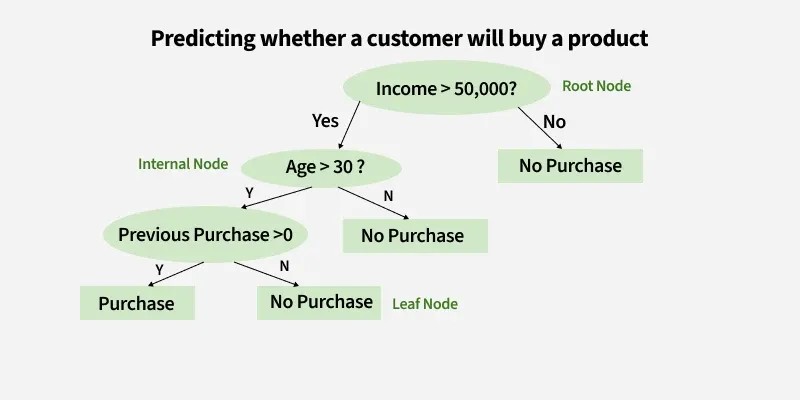
Let’s examine a decision tree designed to forecast whether a customer will purchase a product based on factors like age, income, and previous purchases. Here’s how it operates:

1. Root Node (Income)

First Question: “Is the person’s income greater than $50,000?”
- If Yes, proceed to the next question.
- If No, predict “No Purchase” (leaf node).

2. Internal Node (Age):

If the person’s income exceeds $50,000, ask: “Is the person’s age above 30?”
- If Yes, proceed to the next question.
- If No, predict “No Purchase” (leaf node).

3. Internal Node (Previous Purchases):

If the person is above 30 and has made previous purchases, predict “Purchase” (leaf node).
If the person is above 30 and has not made previous purchases, predict “No Purchase” (leaf node).

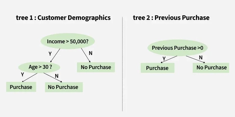
Example: Predicting Whether a Customer Will Buy a Product Using Two Decision Trees

3.1. Tree 1: Customer Demographics

The first tree poses two questions:

“Income > $50,000?”
- If Yes, proceed to the next question.
- If No, predict “No Purchase.”
“Age > 30?”
- Yes: Predict “Purchase.”
- No: Predict “No Purchase.”

3.2. Tree 2: Previous Purchases

“Previous Purchases > 0?”

Yes: Predict “Purchase.”
No: Predict “No Purchase.”

3.3. Combining Trees: Final Prediction

After obtaining predictions from both trees, the results can be combined to arrive at a final prediction. For instance, if Tree 1 predicts “Purchase” and Tree 2 predicts “No Purchase,” the ultimate prediction might be “Purchase” or “No Purchase,” depending on the weight or confidence assigned to each tree. This determination can be made based on the context of the problem.

4. Information Gain and Gini Index in Decision Trees

Now that we have covered the basic intuition and approach of how decision trees work, let’s move to the attribute selection measures.

There are two popular attribute selection measures:

Information Gain
Gini Index

4.1. Information Gain

Information Gain assesses the usefulness of a question (or feature) in dividing data into distinct groups. It gauges the reduction in uncertainty resulting from the split. An effective question yields more distinct groups, and the feature with the highest Information Gain is selected to guide the decision-making process.

For instance, when segmenting a dataset of individuals into “Young” and “Old” categories based on age, if all young individuals purchased the product while none of the old individuals did, the Information Gain would be substantial because the split flawlessly separates the two groups, leaving no residual uncertainty.

Assume that [Tex]S[/Tex] represents a set of instances, [Tex]A [/Tex] stands for an attribute, [Tex]Sv [/Tex] denotes a subset of [Tex]S [/Tex], [Tex]v [/Tex] signifies an individual value that the attribute [Tex]A [/Tex] can assume, and Values ([Tex]A[/Tex]) encompasses the array of possible values for [Tex]A[/Tex]. Then, [Tex]Gain(S, A) = Entropy(S) – sum_{v}^{A}frac{left | S_{v} right |}{left | S right |}. Entropy(S_{v}) [/Tex]
Entropy: Entropy is a measure of the uncertainty of a random variable, which characterizes the impurity of an arbitrary collection of examples. Higher entropy indicates more information content.

For example, if a dataset contains an equal number of “Yes” and “No” outcomes (such as 3 individuals who purchased a product and 3 who did not), the entropy is high because it’s uncertain which outcome to anticipate. Conversely, if all outcomes are uniform (either all “Yes” or all “No”), the entropy is 0, signifying no remaining uncertainty in predicting the outcome.

Assume [Tex]S [/Tex]represents a set of instances, [Tex]A [/Tex] is an attribute, [Tex]Sv [/Tex] is the subset of [Tex]S [/Tex]with [Tex]A [/Tex]= [Tex]v[/Tex], and Values ([Tex]A[/Tex]) is the set of all possible values of [Tex]A[/Tex], then

[Tex]Gain(S, A) = Entropy(S) – sum_{v epsilon Values(A)}frac{left | S_{v} right |}{left | S right |}. Entropy(S_{v}) [/Tex]

Example:

For the set X = {a,a,a,b,b,b,b,b}

Total instances: 8

Instances of b: 5

Instances of a: 3

[Tex]begin{aligned}text{Entropy } H(X) & =left [ left ( frac{3}{8} right )log_{2}frac{3}{8} + left ( frac{5}{8} right )log_{2}frac{5}{8} right ]\& = -[0.375 (-1.415) + 0.625 (-0.678)] \& = -(-0.53-0.424) \& = 0.954end{aligned}[/Tex]

4.2. Building Decision Trees Using Information Gain

Here are the essentials:

Start with all training instances associated with the root node.
Use information gain to choose which attribute to label each node with.
Note: No root-to-leaf path should contain the same discrete attribute twice.
Recursively construct each subtree on the subset of training instances that would be classified down that path in the tree.
If all positive or all negative training instances remain, label that node “yes” or “no” accordingly.
If no attributes remain, label with a majority vote of training instances left at that node.
If no instances remain, label with a majority vote of the parent’s training instances.

Example: Now, let’s draw a Decision Tree for the following data using Information gain.

Training set: 3 features and 2 classes

X	Y	Z	C
1	1	1	I
1	1	0	I
0	0	1	II
1	0	0	II

Here, we have 3 features and 2 output classes. To build a decision tree using Information gain, we will take each of the features and calculate the information for each feature.

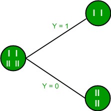
Split on feature X

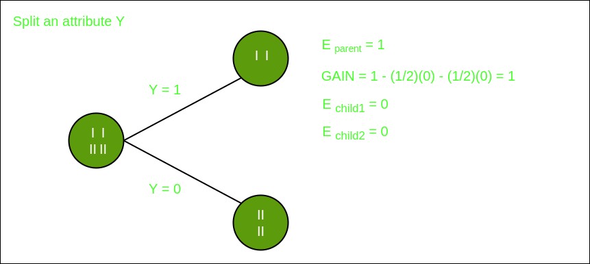
Split on feature Y

Split on feature Z

From the above images, we can see that the information gain is maximum when we make a split on feature Y. So, for the root node the best-suited feature is feature Y. Now we can see that while splitting the dataset by feature Y, the child contains a pure subset of the target variable. So we don’t need to further split the dataset. The final tree for the above dataset would look like this:

4.3. Gini Index

The Gini Index measures how often a randomly chosen element would be incorrectly identified. An attribute with a lower Gini index is preferred.
Scikit-learn supports the “Gini” criterion for the Gini Index, and by default, it takes the “gini” value.

For example, if we have a group of people where all bought the product (100% “Yes”), the Gini Index is 0, indicating perfect purity. But if the group has an equal mix of “Yes” and “No”, the Gini Index would be 0.5, showing higher impurity or uncertainty.

The formula for the Gini Index is:

[Tex]Gini = 1 – sum_{i=1}^{n} p_i^2[/Tex]

Some additional features and characteristics of the Gini Index are:

It is calculated by summing the squared probabilities of each outcome in a distribution and subtracting the result from 1.
A lower Gini Index indicates a more homogeneous or pure distribution, while a higher Gini Index indicates a more heterogeneous or impure distribution.
In decision trees, the Gini Index is used to evaluate the quality of a split by measuring the difference between the impurity of the parent node and the weighted impurity of the child nodes.
Compared to other impurity measures like entropy, the Gini Index is faster to compute and more sensitive to changes in class probabilities.
One disadvantage of the Gini Index is that it tends to favour splits that create equally sized child nodes, even if they are not optimal for classification accuracy.
In practice, the choice between using the Gini Index or other impurity measures depends on the specific problem and dataset, and often requires experimentation and tuning.

5. Real-World Use Case: Understanding Decision Trees Step by Step

We have now grasped the attributes and components of decision trees. Let’s explore a real-life use case to understand how decision trees function step by step.

Step 1. Start with the Whole Dataset

We begin with all the data, treating it as the root node of the decision tree.

Step 2. Choose the Best Question (Attribute)

Pick the best question to divide the dataset. For example, ask: “What is the outlook?”
Possible answers: Sunny, Cloudy, or Rainy.

Step 3. Split the Data into Subsets

Divide the dataset into groups based on the question:
- If Sunny, go to one subset.
- If Cloudy, go to another subset.
- If Rainy, go to the last subset.

Step 4. Split Further if Needed (Recursive Splitting)

For each subset, ask another question to refine the groups. For example:
- If the Sunny subset is mixed, ask: “Is the humidity high or normal?”
  - High humidity → “Swimming”.
  - Normal humidity → “Hiking”.

Step 5. Assign Final Decisions (Leaf Nodes)

When a subset contains only one activity, stop splitting and assign it a label:
- Cloudy → “Hiking”.
- Rainy → “Stay Inside”.
- Sunny + High Humidity → “Swimming”.
- Sunny + Normal Humidity → “Hiking”.

Step 6. Use the Tree for Predictions

To predict an activity, follow the branches of the tree:
- Example: If the outlook is Sunny and the humidity is High, follow the tree:
  - Start at Outlook.
  - Take the branch for Sunny.
  - Then go to Humidity and take the branch for High Humidity.
  - Result: “Swimming”.

This is how a decision tree works: by splitting data step-by-step based on the best questions and stopping when a clear decision is made!

Decision trees provide a powerful and intuitive approach to decision-making, offering both simplicity and interpretability, making them an invaluable tool in the field of machine learning for various classification and regression tasks.

6. Advantages and Disadvantages of Decision Trees

Feature	Decision Trees
Interpretability	Easy to understand and visualize, making them useful for explaining decisions.
Versatility	Can handle both categorical and numerical data.
Non-parametric	No assumptions about the distribution of the data.
Feature Importance	Provides insights into the importance of different features.
Overfitting	Prone to overfitting if the tree is too complex; requires techniques like pruning.
Instability	Small changes in the data can lead to different tree structures.
Bias	Can be biased toward features with more levels.
Optimization	Finding the optimal tree can be computationally expensive.

7. Key Hyperparameters for Decision Tree Optimization

Optimizing a decision tree involves fine-tuning its hyperparameters to achieve the best balance between model complexity and generalization performance. Here’s an overview of the most important hyperparameters:

Hyperparameter	Description	Tuning Effect
Max Depth	Maximum depth of the tree.	Controls the complexity of the tree; lower values prevent overfitting, higher values capture more complex patterns.
Min Samples Split	Minimum number of samples required to split an internal node.	Higher values prevent splits on small subsets, reducing overfitting.
Min Samples Leaf	Minimum number of samples required in a leaf node.	Ensures each leaf node has a minimum number of samples, preventing overfitting.
Criterion	Function used to measure the quality of a split (e.g., Gini impurity, information gain).	Affects how the tree selects the best features to split on. Gini impurity is faster to compute, while information gain is more sensitive to splits.
Max Features	Number of features to consider when looking for the best split.	Reduces overfitting by limiting the number of features considered at each split.
Pruning	Techniques to reduce the size of the tree by removing sections of the tree that provide little power to classify instances.	Helps to prevent overfitting by simplifying the tree.

8. Advanced Techniques and Ensemble Methods

To enhance the performance and robustness of decision trees, advanced techniques and ensemble methods can be employed. Here’s an exploration of these approaches:

8.1. Ensemble Methods

Ensemble methods combine multiple decision trees to make more accurate predictions. Two popular ensemble methods are:

Random Forest: Random Forest constructs a multitude of decision trees during training. Each tree is built on a random subset of the data and features. The final prediction is made by averaging or voting the predictions of individual trees, reducing overfitting and improving accuracy.
Gradient Boosting: Gradient Boosting builds trees sequentially, where each tree corrects the errors of the previous one. It combines weak learners into a strong learner by minimizing a loss function. Popular gradient boosting algorithms include XGBoost, LightGBM, and CatBoost.

8.2. Pruning Techniques

Pruning techniques are used to reduce the size of the decision tree by removing branches that provide little predictive power. This helps to prevent overfitting and improve the generalization performance of the tree. Common pruning techniques include:

Cost Complexity Pruning (CCP): CCP prunes the tree based on a complexity parameter that penalizes trees with more nodes.
Reduced Error Pruning: Reduced Error Pruning removes nodes if their removal does not significantly increase the error on a validation set.

8.3. Handling Imbalanced Data

Imbalanced data occurs when one class is much more frequent than the other. Decision trees can be biased towards the majority class in such cases. Techniques to handle imbalanced data include:

Oversampling: Oversampling techniques like SMOTE (Synthetic Minority Oversampling Technique) generate synthetic samples for the minority class to balance the dataset.
Undersampling: Undersampling techniques reduce the number of samples in the majority class to balance the dataset.
Cost-Sensitive Learning: Cost-sensitive learning assigns higher costs to misclassifying the minority class, forcing the decision tree to pay more attention to it.

8.4. Feature Engineering

Feature engineering involves creating new features from existing ones to improve the performance of the decision tree. This can include:

Polynomial Features: Adding polynomial terms of existing features.
Interaction Features: Creating new features by combining two or more existing features.
Domain-Specific Features: Creating features based on domain knowledge that are relevant to the problem.

9. Frequently Asked Questions (FAQs)

9.1. What are the Major Issues in Decision Tree Learning?

Major issues in decision tree learning include overfitting, sensitivity to small data changes, and limited generalization. Ensuring proper pruning, tuning, and handling imbalanced data can help mitigate these challenges for more robust decision tree models.

9.2. How Does a Decision Tree Help in Decision Making?

Decision trees aid decision-making by representing complex choices in a hierarchical structure. Each node tests specific attributes, guiding decisions based on data values. Leaf nodes provide final outcomes, offering a clear and interpretable path for decision analysis in machine learning.

9.3. What is the Maximum Depth of a Decision Tree?

The maximum depth of a decision tree is a hyperparameter that determines the maximum number of levels or nodes from the root to any leaf. It controls the complexity of the tree and helps prevent overfitting.

9.4. What is the Concept of a Decision Tree?

A decision tree is a supervised learning algorithm that models decisions based on input features. It forms a tree-like structure where each internal node represents a decision based on an attribute, leading to leaf nodes representing outcomes.

9.5. What is Entropy in a Decision Tree?

In decision trees, entropy is a measure of impurity or disorder within a dataset. It quantifies the uncertainty associated with classifying instances, guiding the algorithm to make informative splits for effective decision-making.

9.6. What are the Hyperparameters of a Decision Tree?

Max Depth: Maximum depth of the tree.

Min Samples Split: Minimum samples required to split an internal node.

Min Samples Leaf: Minimum samples required in a leaf node.

Criterion: The function used to measure the quality of a split.

10. Ready to Learn More?

Unlock your potential with LEARNS.EDU.VN. Explore in-depth articles, comprehensive guides, and tailored courses designed to enhance your understanding and skills in machine learning. Whether you’re a student, a professional, or simply curious, we have the resources you need to succeed.

Overcome your learning challenges with our clear, reliable, and expertly crafted educational materials. Our resources are designed to simplify complex concepts, making learning enjoyable and effective.

Don’t miss out on the opportunity to gain a competitive edge. Visit learns.edu.vn today and discover a world of knowledge at your fingertips.

Contact us:

Address: 123 Education Way, Learnville, CA 90210, United States
WhatsApp: +1 555-555-1212
Website: LEARNS.EDU.VN

Start your learning journey now and transform your future with us.