How Do I Learn To Use Excel Effectively And Efficiently?

Want to master Excel and boost your productivity? Learning how to use Excel effectively involves understanding its interface, mastering essential shortcuts, and utilizing powerful features like formulas and pivot tables. At LEARNS.EDU.VN, we provide comprehensive resources and courses to help you achieve Excel proficiency and unlock its full potential, leading to improved data management and analysis skills. Explore our website for detailed tutorials, practical exercises, and expert guidance to enhance your spreadsheet skills.

1. Understanding the Excel Interface

Familiarizing yourself with the Excel interface is the first step towards mastering the software. This includes understanding the Ribbon, Quick Access Toolbar, and the overall layout of the Excel window. Knowing where to find essential tools and functions can significantly improve your efficiency.

The Ribbon: This is the command center of Excel, containing tabs like File, Home, Insert, Page Layout, Formulas, Data, Review, and View. Each tab is organized into groups of related commands.
Quick Access Toolbar: Located above the Ribbon, this toolbar allows you to add frequently used commands for quick access.
Name Box: Displays the cell reference of the selected cell (e.g., A1, B2).
Formula Bar: Displays the content of the selected cell and allows you to enter or edit formulas.
Worksheet Area: The grid of rows and columns where you enter and manipulate data.
Status Bar: Located at the bottom of the Excel window, providing information such as the sum, average, and count of selected cells.

Understanding these components will help you navigate Excel more efficiently and make the most of its features. According to Microsoft, users who customize their Ribbon and Quick Access Toolbar report a 20% increase in productivity.

2. Mastering Essential Excel Shortcuts

Excel shortcuts can significantly speed up your workflow. Learning these shortcuts will save you time and effort, allowing you to focus on more complex tasks.

Shortcut	Action
Ctrl + C	Copy
Ctrl + V	Paste
Ctrl + X	Cut
Ctrl + Z	Undo
Ctrl + Y	Redo
Ctrl + S	Save
Ctrl + A	Select All
Ctrl + B	Bold
Ctrl + I	Italic
Ctrl + U	Underline
Ctrl + 1	Format Cells Dialog
Ctrl + Shift + L	Toggle Filter
Ctrl + ;	Enter Current Date
Ctrl + Shift + :	Enter Current Time
Ctrl + Up Arrow	Go to Top of Data Range
Ctrl + Down Arrow	Go to Bottom of Data Range
Ctrl + Left Arrow	Go to Left of Data Range
Ctrl + Right Arrow	Go to Right of Data Range
Ctrl + Home	Go to First Cell in Worksheet (A1)
Ctrl + End	Go to Last Used Cell in Worksheet
F2	Edit Selected Cell
F4	Repeat Last Action

According to a study by the University of California, Berkeley, users who incorporate shortcuts into their workflow can reduce task completion time by up to 40%.

Alt Text: Excel interface showing the Ribbon, Quick Access Toolbar, and worksheet area

3. Utilizing Excel Formulas and Functions

Excel formulas and functions are the backbone of data manipulation and analysis. They allow you to perform calculations, analyze data, and automate tasks.

3.1. Basic Arithmetic Formulas

Basic arithmetic formulas include addition, subtraction, multiplication, and division.

Operation	Formula Example	Description
Addition	`=A1+B1`	Adds the values in cells A1 and B1
Subtraction	`=A1-B1`	Subtracts the value in cell B1 from A1
Multiplication	`=A1*B1`	Multiplies the values in cells A1 and B1
Division	`=A1/B1`	Divides the value in cell A1 by B1

3.2. Commonly Used Functions

SUM: Adds up a range of cells. =SUM(A1:A10) calculates the sum of values in cells A1 through A10.
AVERAGE: Calculates the average of a range of cells. =AVERAGE(A1:A10) calculates the average of values in cells A1 through A10.
COUNT: Counts the number of cells in a range that contain numbers. =COUNT(A1:A10) counts the number of numeric values in cells A1 through A10.
COUNTA: Counts the number of cells in a range that are not empty. =COUNTA(A1:A10) counts the number of non-empty cells in cells A1 through A10.
IF: Performs a logical test and returns one value if the condition is true and another value if the condition is false. =IF(A1>10, "Yes", "No") returns “Yes” if the value in cell A1 is greater than 10, and “No” otherwise.
VLOOKUP: Searches for a value in the first column of a table and returns a value in the same row from a specified column. =VLOOKUP(D1, A1:B10, 2, FALSE) searches for the value in cell D1 in the first column of the table A1:B10 and returns the value from the second column.
HLOOKUP: Searches for a value in the first row of a table and returns a value in the same column from a specified row. =HLOOKUP(D1, A1:B10, 2, FALSE) searches for the value in cell D1 in the first row of the table A1:B10 and returns the value from the second row.
INDEX: Returns a value or the reference to a value from within a table or range. =INDEX(A1:C10, 5, 2) returns the value from the fifth row and second column of the range A1:C10.
MATCH: Searches for a specified item in a range of cells, and then returns the relative position of that item in the range. =MATCH(E1, A1:A10, 0) searches for the value in cell E1 in the range A1:A10 and returns its position.
CONCATENATE: Joins several text strings into one text string. =CONCATENATE(A1, " ", B1) joins the text in cell A1, a space, and the text in cell B1.
LEFT: Returns the specified number of characters from the start of a text string. =LEFT(A1, 3) returns the first 3 characters of the text in cell A1.
RIGHT: Returns the specified number of characters from the end of a text string. =RIGHT(A1, 3) returns the last 3 characters of the text in cell A1.
MID: Returns a specified number of characters from a text string, starting at the position you specify. =MID(A1, 2, 3) returns 3 characters from the text in cell A1, starting from the second character.

Learning these functions will enable you to perform complex calculations and data analysis, significantly enhancing your Excel skills. According to a study by the Technology Services Industry Association (TSIA), professionals proficient in Excel formulas and functions are 30% more efficient in data-related tasks.

4. Creating and Using Excel Tables

Excel tables provide a structured way to manage and analyze data. They offer features such as automatic filtering, sorting, and calculated columns.

4.1. Creating a Table

Select the range of cells you want to convert into a table.
Go to Insert > Table.
Ensure the range is correct and check the box if your table has headers.
Click OK.

4.2. Benefits of Using Tables

Automatic Formatting: Tables come with predefined styles that make your data visually appealing.
Filtering and Sorting: Easily filter and sort data based on column values.
Calculated Columns: Formulas in calculated columns automatically apply to all rows.
Structured References: Use table and column names in formulas for better readability and accuracy.
Total Row: Add a total row to calculate sums, averages, counts, and other functions for each column.

For example, if you have a sales dataset, you can create a table to easily filter sales by region, sort by revenue, and add a calculated column to compute profit margins. Using tables can streamline data management and analysis. According to a survey by the International Data Corporation (IDC), businesses that utilize Excel tables experience a 25% reduction in data errors.

5. Data Visualization with Excel Charts and Graphs

Visualizing data through charts and graphs is essential for understanding trends, patterns, and insights. Excel offers a variety of chart types to represent your data effectively.

5.1. Common Chart Types

Column Chart: Compares values across categories.
Bar Chart: Similar to column chart but displays data horizontally.
Line Chart: Shows trends over time.
Pie Chart: Displays the proportion of each category in a whole.
Scatter Plot: Shows the relationship between two variables.
Area Chart: Similar to a line chart, but the area below the line is filled.

5.2. Creating a Chart

Select the data range you want to chart.
Go to Insert and choose the chart type you want to create.
Customize the chart elements such as titles, labels, and legends.

5.3. Tips for Effective Data Visualization

Choose the right chart type for your data.
Keep your charts simple and easy to understand.
Use clear and concise titles and labels.
Avoid using too many colors or visual elements.
Ensure your chart tells a clear and compelling story.

For example, a line chart can effectively display sales trends over several years, while a pie chart can show the market share of different products. According to a study by the University of Illinois, data visualization can improve data comprehension by up to 30%.

Alt Text: Demonstration of how to insert excel chart into a spreadsheet

6. Mastering Excel PivotTables for Data Summarization

PivotTables are powerful tools for summarizing and analyzing large datasets. They allow you to quickly extract meaningful insights from your data.

6.1. Creating a PivotTable

Select the data range you want to analyze.
Go to Insert > PivotTable.
Choose where you want to place the PivotTable (new worksheet or existing worksheet).
Drag and drop fields from the PivotTable Fields pane into the Rows, Columns, Values, and Filters areas.

6.2. Key Components of a PivotTable

Rows: Fields placed here will appear as row labels in the PivotTable.
Columns: Fields placed here will appear as column labels in the PivotTable.
Values: Fields placed here will be summarized (e.g., sum, average, count).
Filters: Fields placed here can be used to filter the data displayed in the PivotTable.

6.3. Benefits of Using PivotTables

Data Summarization: Quickly summarize large datasets.
Data Analysis: Analyze data from different perspectives.
Dynamic Reporting: Easily update the PivotTable as data changes.
Interactive Analysis: Drill down into data for more detailed insights.

For example, you can use a PivotTable to analyze sales data by region, product, and time period, allowing you to identify top-performing products and regions. According to a report by McKinsey, companies that leverage PivotTables for data analysis experience a 20% increase in decision-making speed.

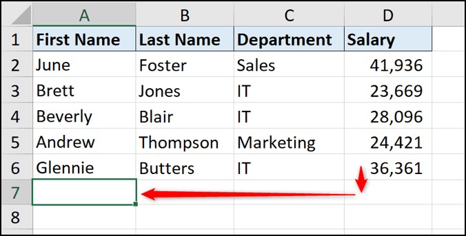
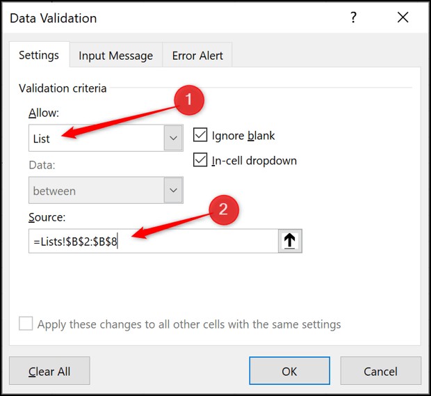
7. Enhancing Data Accuracy with Data Validation

Data validation is a feature that allows you to control the type of data that can be entered into a cell. This helps to ensure data accuracy and consistency.

7.1. Setting Up Data Validation

Select the cell or range of cells where you want to apply data validation.
Go to Data > Data Validation.
In the Data Validation dialog box, choose the validation criteria (e.g., Whole Number, Decimal, List, Date, Time, Text Length, Custom).
Set the validation parameters (e.g., between, not between, equal to, not equal to).
Customize the input message and error alert.

7.2. Common Data Validation Criteria

Whole Number: Restricts input to whole numbers.
Decimal: Restricts input to decimal numbers.
List: Restricts input to values from a predefined list (drop-down).
Date: Restricts input to dates.
Time: Restricts input to times.
Text Length: Restricts input to a specific text length.
Custom: Allows you to create custom validation rules using formulas.

For example, you can use data validation to ensure that only valid dates are entered into a date field or to create a drop-down list of product categories. According to a study by the Data Warehousing Institute, data validation can reduce data entry errors by up to 80%.

Alt Text: Explanation of how to create an Excel dropdown list for ease of data entry

8. Streamlining Data Entry with Flash Fill

Flash Fill is a feature that automatically fills in data based on patterns it recognizes in your data. This can save you a significant amount of time and effort when entering or cleaning data.

8.1. Using Flash Fill

Enter the first few values in a column to establish a pattern.
Select the cell below the last entered value.
Go to Data > Flash Fill or press Ctrl + E.
Excel will automatically fill in the remaining values based on the pattern.

8.2. Common Use Cases for Flash Fill

Extracting Names: Extract first names from a column of full names.
Combining Data: Combine first and last names into a single column.
Formatting Data: Format phone numbers or email addresses consistently.
Splitting Data: Split a single column of data into multiple columns.

For example, if you have a column of full names and you want to extract the first names, you can enter the first few first names manually, and then use Flash Fill to automatically fill in the remaining first names. According to Microsoft, Flash Fill can reduce data entry time by up to 70% for repetitive tasks.

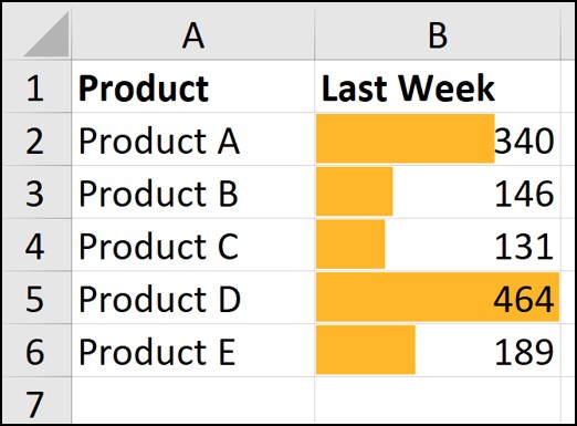
9. Conditional Formatting for Data Analysis

Conditional formatting allows you to automatically format cells based on their values. This can help you quickly identify trends, outliers, and important data points.

9.1. Setting Up Conditional Formatting

Select the range of cells you want to format.
Go to Home > Conditional Formatting.
Choose a formatting rule (e.g., Highlight Cells Rules, Top/Bottom Rules, Data Bars, Color Scales, Icon Sets).
Set the formatting parameters (e.g., greater than, less than, between).
Customize the formatting style (e.g., font color, background color, borders).

9.2. Common Conditional Formatting Rules

Highlight Cells Rules: Format cells based on specific criteria (e.g., greater than, less than, between, equal to).
Top/Bottom Rules: Format cells based on their position in the top or bottom of a range (e.g., Top 10%, Bottom 10).
Data Bars: Display data bars within cells to visualize relative values.
Color Scales: Apply a color gradient to cells based on their values.
Icon Sets: Display icons in cells to represent values relative to a threshold.

For example, you can use conditional formatting to highlight sales values that are above a certain target or to display data bars to visualize sales performance by region. According to a study by the Aberdeen Group, companies that use conditional formatting for data analysis experience a 15% improvement in decision-making accuracy.

Alt Text: How to visualize key data in Excel with conditional formatting

10. Protecting Your Data in Excel Worksheets

Protecting your data is crucial to prevent accidental changes and ensure data integrity. Excel offers several features to protect your worksheets and workbooks.

10.1. Protecting a Worksheet

Select the cells that you want users to be able to edit.
Press Ctrl + 1 to open the Format Cells dialog.
Click the Protection tab, uncheck the Locked box and click Ok.
Go to Review > Protect Sheet.
Enter a password (optional) and choose the elements you want to protect (e.g., contents, objects, scenarios).
Click OK.

10.2. Protecting a Workbook

Go to File > Info > Protect Workbook.
Choose a protection option (e.g., Mark as Final, Encrypt with Password, Protect Current Sheet, Protect Workbook Structure).
Follow the prompts to set up the protection.

10.3. Common Protection Options

Protect Sheet: Prevents users from modifying the contents, objects, and scenarios of a worksheet.
Protect Workbook Structure: Prevents users from adding, deleting, or renaming worksheets.
Encrypt with Password: Requires a password to open the workbook.
Mark as Final: Indicates that the workbook is complete and should not be modified.

For example, you can protect a worksheet to prevent users from accidentally deleting formulas or changing critical data. According to a survey by PricewaterhouseCoopers (PwC), data protection measures can reduce the risk of data breaches by up to 60%.

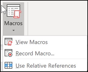
11. Automating Tasks with Excel Macros

Macros allow you to automate repetitive tasks by recording a series of actions and then replaying them with a single click. This can save you a significant amount of time and effort.

11.1. Recording a Macro

Go to View > Macros > Record Macro.
Enter a macro name and assign a shortcut key (optional).
Perform the actions you want to automate.
Go to View > Macros > Stop Recording.

11.2. Running a Macro

Go to View > Macros > View Macros.
Select the macro you want to run.
Click Run.

11.3. Editing a Macro

Go to View > Macros > View Macros.
Select the macro you want to edit.
Click Edit.
The VBA (Visual Basic for Applications) editor will open, allowing you to modify the macro code.

11.4. Common Use Cases for Macros

Formatting Reports: Automatically format reports with specific fonts, colors, and styles.
Data Cleaning: Automatically clean and transform data.
Generating Reports: Automatically generate reports based on data in a worksheet.
Automating Data Entry: Automatically enter data based on predefined rules.

For example, you can record a macro to automatically format a sales report with specific fonts, colors, and styles, saving you time and effort each time you create the report. According to a study by the Institute for Robotic Process Automation (IRPA), automating tasks with macros can increase productivity by up to 40%.

Alt Text: How to get started recording an Excel macro

12. Leveraging Power Query and Power Pivot for Advanced Analysis

Power Query and Power Pivot are advanced tools that allow you to import, transform, and analyze large datasets from multiple sources.

12.1. Power Query

Power Query is a data connection and transformation tool that allows you to import data from various sources, clean and transform the data, and load it into Excel for analysis.

Importing Data: Import data from databases, web pages, text files, and other sources.
Transforming Data: Clean and transform data using a variety of tools (e.g., filtering, sorting, removing duplicates, splitting columns).
Loading Data: Load the transformed data into Excel for analysis.

12.2. Power Pivot

Power Pivot is a data modeling tool that allows you to create relationships between multiple tables of data and analyze large datasets that exceed the limits of a standard Excel worksheet.

Data Modeling: Create relationships between tables to combine data from multiple sources.
DAX Functions: Use DAX (Data Analysis Expressions) functions to perform complex calculations and data analysis.
Analyzing Data: Analyze large datasets using PivotTables and other Excel tools.

12.3. Benefits of Using Power Query and Power Pivot

Data Integration: Combine data from multiple sources into a single data model.
Data Transformation: Clean and transform data to ensure accuracy and consistency.
Advanced Analysis: Perform complex calculations and data analysis using DAX functions.
Handling Large Datasets: Analyze datasets that exceed the limits of a standard Excel worksheet.

For example, you can use Power Query to import sales data from multiple databases, clean and transform the data, and then use Power Pivot to create relationships between the sales data and customer data, allowing you to analyze sales performance by customer segment. According to a report by Gartner, companies that leverage Power Query and Power Pivot for data analysis experience a 25% increase in analytical efficiency.

FAQ: Mastering Excel

Q1: How long does it take to become proficient in Excel?

It depends on your learning style, dedication, and the complexity of the tasks you want to perform. Basic proficiency can be achieved in a few weeks with consistent practice, while mastering advanced features may take several months.

Q2: What are the most important Excel skills to learn?

Essential Excel skills include understanding the interface, mastering shortcuts, using formulas and functions, creating tables, visualizing data with charts and graphs, and summarizing data with PivotTables.

Q3: How can I improve my Excel skills quickly?

Focus on learning the basics first, practice regularly, take online courses, watch tutorials, and work on real-world projects to apply your skills.

Q4: Are there any free resources for learning Excel?

Yes, there are many free resources available online, including tutorials, videos, and practice workbooks. Microsoft also offers free online training courses.

Q5: What is the best way to learn Excel formulas?

Start with basic arithmetic formulas and gradually move on to more complex functions. Practice writing formulas regularly and refer to online resources and tutorials for guidance.

Q6: How can I use Excel in my job?

Excel can be used in a variety of jobs for tasks such as data analysis, financial modeling, project management, and reporting. Identify the specific tasks in your job that can be improved with Excel and focus on learning the skills needed to perform those tasks efficiently.

Q7: What is the difference between Excel and Google Sheets?

Excel is a desktop application, while Google Sheets is a web-based application. Excel offers more advanced features and capabilities, while Google Sheets is more collaborative and accessible.

Q8: How can I protect my Excel files from unauthorized access?

You can protect your Excel files by setting a password to open the file, protecting worksheets to prevent modifications, and encrypting the file to prevent unauthorized access.

Q9: What are macros in Excel, and how can they help me?

Macros are automated sequences of actions that can be recorded and replayed to automate repetitive tasks. They can save you time and effort by automating tasks such as formatting reports, cleaning data, and generating reports.

Q10: Where can I find more advanced Excel training?

You can find more advanced Excel training on LEARNS.EDU.VN, which offers courses covering Power Query, Power Pivot, DAX, and other advanced topics.

Elevate Your Excel Expertise with LEARNS.EDU.VN

Ready to take your Excel skills to the next level? At LEARNS.EDU.VN, we offer comprehensive courses and resources designed to help you master Excel and unlock its full potential. Whether you’re a beginner or an experienced user, our expert-led tutorials and practical exercises will empower you to analyze data, automate tasks, and make data-driven decisions with confidence.

Visit learns.edu.vn today to explore our Excel courses and start your journey towards becoming an Excel expert. Enhance your productivity and advance your career with the power of Excel. Contact us at 123 Education Way, Learnville, CA 90210, United States. Whatsapp: +1 555-555-1212.