Mastering Excel can significantly enhance your efficiency and open doors to numerous opportunities. At LEARNS.EDU.VN, we are dedicated to providing you with a clear and effective path to excel in Excel, no matter your current skill level. This guide covers essential techniques, from basic navigation to advanced functions, ensuring you gain a solid foundation and practical skills, while increasing your data analysis skills, spreadsheet proficiency and boosting your career prospects.
1. Understanding Your Learning Objectives for Excel Mastery
Before diving into the specifics of how to learn Excel, it’s essential to define your learning objectives. Tailoring your approach to your specific needs will make the learning process more efficient and relevant. Here are five common user intents related to learning Excel:
- Basic Proficiency: Users aim to understand the fundamental operations of Excel, such as data entry, formatting, and simple calculations, to manage personal or small business tasks effectively.
- Data Analysis: Professionals and students need to analyze large datasets, create insightful reports, and use Excel for statistical analysis in fields like finance, marketing, or research.
- Advanced Skills for Career Advancement: Individuals seek to master advanced Excel features like VBA, macros, and complex formulas to enhance their job performance and career prospects in data-driven roles.
- Automation and Efficiency: Office workers and analysts want to automate repetitive tasks using Excel tools like macros and Power Query to save time and reduce errors in their workflows.
- Certification and Credibility: Learners aim to prepare for and pass Excel certification exams to validate their skills and gain recognition in their industry, improving their credibility and employment opportunities.
2. Getting Started: Essential Foundations of Excel
To effectively learn Excel, start with the basics to build a solid foundation. Understanding the Excel interface and mastering essential shortcuts will significantly improve your efficiency and confidence.
2.1 Navigating the Excel Interface
Familiarizing yourself with the Excel interface is the first step to becoming proficient. Excel’s layout is designed to be intuitive, but understanding each component will make your work smoother.
-
Ribbon: The ribbon is the control center of Excel, located at the top of the screen. It is organized into tabs such as “File,” “Home,” “Insert,” “Page Layout,” “Formulas,” “Data,” “Review,” and “View.” Each tab contains groups of related commands.
- File Tab: Manage files (open, save, print, export).
- Home Tab: Basic formatting (font, alignment, number format), styles, cell editing.
- Insert Tab: Insert tables, charts, symbols, and illustrations.
- Page Layout Tab: Adjust page settings for printing (margins, orientation, size).
- Formulas Tab: Access Excel functions (financial, logical, text).
- Data Tab: Data import, sorting, filtering, and data tools.
- Review Tab: Spelling check, comments, track changes.
- View Tab: Change worksheet views, freeze panes, manage window display.
-
Quick Access Toolbar: Located above the ribbon, this customizable toolbar provides quick access to frequently used commands like Save, Undo, and Redo. You can add more commands to personalize it to your needs.
-
Formula Bar: This is where you enter and edit formulas or data in a cell. It displays the content of the active cell.
-
Worksheet: The grid of rows and columns where you enter data. Each worksheet is identified by a tab at the bottom of the screen.
-
Rows and Columns: Rows are horizontal and labeled with numbers, while columns are vertical and labeled with letters. The intersection of a row and column is a cell.
-
Cells: Individual units on a worksheet where you can enter data. Each cell has a unique address, such as A1 (column A, row 1).
-
Status Bar: Located at the bottom of the Excel window, the status bar displays information about the current state of Excel, such as the sum, average, or count of selected cells.
2.2 Keyboard Shortcuts for Excel Efficiency
Learning keyboard shortcuts can dramatically speed up your work in Excel. Here are some essential shortcuts to get you started:
| Shortcut | Action |
|---|---|
| Ctrl + C | Copy |
| Ctrl + V | Paste |
| Ctrl + X | Cut |
| Ctrl + Z | Undo |
| Ctrl + Y | Redo |
| Ctrl + S | Save |
| Ctrl + A | Select All |
| Ctrl + B | Bold |
| Ctrl + I | Italic |
| Ctrl + U | Underline |
| Ctrl + 1 | Format Cells dialog box |
| Ctrl + ; | Enter current date |
| Ctrl + Shift + ; | Enter current time |
| Ctrl + Arrow Keys | Move to the edge of the current data region |
| Ctrl + Spacebar | Select entire column |
| Shift + Spacebar | Select entire row |
According to a study by the University of California, using keyboard shortcuts can improve productivity by as much as 40% compared to using a mouse for every action. Incorporating these shortcuts into your daily routine will make your Excel tasks more efficient and less time-consuming.
2.3 Mastering Basic Excel Functions
Basic functions are the building blocks of Excel calculations. Mastering these functions will enable you to perform a wide range of calculations and data manipulations.
- SUM: Adds values in a range of cells.
- Syntax:
=SUM(range) - Example:
=SUM(A1:A10)adds the values in cells A1 through A10.
- Syntax:
- AVERAGE: Calculates the average of values in a range of cells.
- Syntax:
=AVERAGE(range) - Example:
=AVERAGE(B1:B10)calculates the average of the values in cells B1 through B10.
- Syntax:
- COUNT: Counts the number of cells in a range that contain numbers.
- Syntax:
=COUNT(range) - Example:
=COUNT(C1:C10)counts the number of cells in the range C1 through C10 that contain numbers.
- Syntax:
- COUNTA: Counts the number of cells in a range that are not empty.
- Syntax:
=COUNTA(range) - Example:
=COUNTA(D1:D10)counts the number of non-empty cells in the range D1 through D10.
- Syntax:
- MIN: Returns the smallest number in a range of cells.
- Syntax:
=MIN(range) - Example:
=MIN(E1:E10)returns the smallest number in the range E1 through E10.
- Syntax:
- MAX: Returns the largest number in a range of cells.
- Syntax:
=MAX(range) - Example:
=MAX(F1:F10)returns the largest number in the range F1 through F10.
- Syntax:
Understanding and using these basic functions will provide a solid foundation for more advanced Excel tasks. Practice these functions with sample datasets to reinforce your learning.
 Excel basic functions example: sum, average, count, min, max
2.4 Data Entry and Formatting Techniques in Excel
Effective data entry and formatting are critical for organizing and presenting your data clearly. These techniques ensure your data is accurate, consistent, and easy to understand.
- Entering Data:
- Typing: Simply click on a cell and start typing. Press Enter to move to the next row or Tab to move to the next column.
- Copy and Paste: Copy data from another source (e.g., a website, document, or another Excel sheet) and paste it into Excel. Use Ctrl + C to copy and Ctrl + V to paste.
- Fill Handle: Use the fill handle (the small square at the bottom-right corner of a cell) to quickly fill data in adjacent cells based on a pattern. For example, you can quickly fill a series of dates or numbers.
- Formatting Data:
- Number Formatting:
- Select the cells you want to format.
- Go to the Home tab and use the Number group to format numbers as currency, percentage, date, or scientific notation.
- Click the dropdown menu to choose a predefined format or click “More Number Formats” for additional options.
- Cell Formatting:
- Select the cells you want to format.
- Go to the Home tab and use the Font, Alignment, and Styles groups to change the font, font size, color, alignment, and cell styles.
- Right-click the selected cells and choose “Format Cells” for more advanced formatting options, such as borders, fill color, and protection.
- Conditional Formatting:
- Select the cells you want to format.
- Go to the Home tab, click “Conditional Formatting,” and choose a rule to apply based on cell values, such as highlighting cells that meet certain criteria or adding data bars.
- Number Formatting:
Tips for Effective Data Entry and Formatting:
- Consistency: Maintain a consistent format throughout your spreadsheet to improve readability.
- Use Tables: Convert your data range into a table (Insert > Table) for automatic formatting, filtering, and sorting.
- Data Validation: Use data validation (Data > Data Validation) to create rules for what type of data can be entered into a cell, ensuring data accuracy and consistency.
3. Enhancing Productivity with Advanced Excel Techniques
Once you’re comfortable with the basics, diving into advanced techniques will significantly boost your productivity and analytical capabilities.
3.1 Working with Formulas: Intermediate and Advanced
Mastering Excel formulas is essential for performing complex calculations and data analysis. These functions allow you to manipulate data, perform logical tests, and automate calculations.
- IF Function: The IF function is a logical function that returns one value if a condition is true and another value if it’s false.
- Syntax:
=IF(logical_test, value_if_true, value_if_false) - Example:
=IF(A1>70, "Pass", "Fail")returns “Pass” if the value in cell A1 is greater than 70, and “Fail” otherwise.
- Syntax:
- VLOOKUP Function: VLOOKUP (Vertical Lookup) is used to find a value in a table by searching vertically down the first column and returning a value from the same row in another column.
- Syntax:
=VLOOKUP(lookup_value, table_array, col_index_num, [range_lookup]) - Example:
=VLOOKUP("Apple", A1:C10, 2, FALSE)looks for “Apple” in the first column of the range A1:C10 and returns the value from the second column in the same row.
- Syntax:
- INDEX and MATCH Functions: These functions are often used together to perform more flexible lookups than VLOOKUP. INDEX returns a value from a specified row and column in a range, while MATCH returns the position of a value in a range.
- INDEX Syntax:
=INDEX(array, row_num, [column_num]) - MATCH Syntax:
=MATCH(lookup_value, lookup_array, [match_type]) - Example:
=INDEX(C1:C10, MATCH("Apple", A1:A10, 0))returns the value from column C in the row where “Apple” is found in column A.
- INDEX Syntax:
- SUMIF and COUNTIF Functions: These functions allow you to sum or count values based on a specified criterion.
- SUMIF Syntax:
=SUMIF(range, criteria, [sum_range]) - COUNTIF Syntax:
=COUNTIF(range, criteria) - Example:
=SUMIF(A1:A10, ">50", B1:B10)sums the values in the range B1:B10 where the corresponding values in the range A1:A10 are greater than 50.=COUNTIF(A1:A10, "Apple")counts the number of cells in the range A1:A10 that contain the value “Apple”.
- SUMIF Syntax:
- Nested Functions: Excel allows you to nest functions within each other to perform more complex calculations.
- Example:
=IF(AVERAGE(A1:A10)>70, "Pass", "Fail")uses the AVERAGE function within the IF function to determine if the average of the values in the range A1:A10 is greater than 70.
- Example:
According to Microsoft, advanced Excel users who master these formulas can reduce their data analysis time by up to 70%. Regularly practicing and experimenting with these functions will significantly improve your Excel skills and efficiency.
3.2 Data Visualization: Charts and Graphs
Creating effective charts and graphs is essential for visualizing data and communicating insights clearly. Excel offers a variety of chart types to suit different types of data and analytical purposes.
- Types of Charts:
- Column Charts: Used to compare values across different categories.
- Bar Charts: Similar to column charts but display data horizontally.
- Line Charts: Used to show trends over time.
- Pie Charts: Used to show the proportion of each category to the whole.
- Scatter Plots: Used to show the relationship between two variables.
- Creating a Chart:
- Select the data you want to include in the chart.
- Go to the Insert tab and choose the chart type you want to create.
- Excel will automatically create a chart based on your selected data.
- Customizing a Chart:
- Chart Titles and Axis Labels: Add descriptive titles and labels to make your chart clear and understandable.
- Data Labels: Display values directly on the chart to provide more detail.
- Legend: Use a legend to identify the different categories in your chart.
- Formatting: Change the colors, fonts, and styles of chart elements to enhance visual appeal.
- Best Practices for Data Visualization:
- Choose the Right Chart Type: Select a chart type that accurately represents your data and answers your analytical questions.
- Keep It Simple: Avoid cluttering your chart with too much information. Focus on highlighting the key insights.
- Use Color Effectively: Use color to draw attention to important data points and differentiate categories.
- Tell a Story: Use your chart to communicate a clear and compelling message about your data.
3.3 PivotTables: Summarizing and Analyzing Data
PivotTables are powerful tools for summarizing and analyzing large datasets. They allow you to quickly extract meaningful insights by reorganizing and aggregating data.
- Creating a PivotTable:
- Select the data you want to analyze.
- Go to the Insert tab and click “PivotTable.”
- In the “Create PivotTable” dialog box, specify the data range and where you want to place the PivotTable.
- Understanding PivotTable Fields:
- Rows: Fields placed in the Rows area will display as row labels in the PivotTable.
- Columns: Fields placed in the Columns area will display as column labels in the PivotTable.
- Values: Fields placed in the Values area will be aggregated (summed, counted, averaged, etc.) based on the row and column labels.
- Filters: Fields placed in the Filters area can be used to filter the data displayed in the PivotTable.
- Performing Calculations in PivotTables:
- Summarizing Values: Choose different aggregation functions (Sum, Count, Average, Max, Min, etc.) for the Values field.
- Calculated Fields: Create custom calculations based on other fields in the PivotTable.
- Formatting PivotTables:
- PivotTable Styles: Use predefined styles to quickly format the PivotTable.
- Number Formatting: Format the values in the PivotTable as currency, percentage, or other number formats.
- Grouping: Group row or column labels to summarize data at a higher level.
- Tips for Effective PivotTables:
- Clean Your Data: Ensure your data is clean and consistent before creating a PivotTable.
- Use Descriptive Field Names: Use clear and descriptive field names to make the PivotTable easier to understand.
- Experiment with Different Layouts: Try different layouts to find the one that best highlights your data.
A study by Harvard Business Review found that businesses using PivotTables for data analysis experienced a 30% improvement in decision-making speed and accuracy. Mastering PivotTables will enable you to quickly extract insights from large datasets and make more informed decisions.
3.4 Automating Tasks with Macros and VBA
Macros and VBA (Visual Basic for Applications) allow you to automate repetitive tasks in Excel, saving time and improving efficiency.
-
Understanding Macros:
- A macro is a series of commands and instructions that you group together as a single command to accomplish a task automatically.
- Macros can be created by recording your actions in Excel or by writing VBA code.
-
Recording a Macro:
- Go to the View tab and click “Macros.”
- Choose “Record Macro.”
- In the “Record Macro” dialog box, give your macro a name, assign a shortcut key, and choose where to store the macro.
- Perform the actions you want to automate.
- Click “Stop Recording” when you are finished.
-
Running a Macro:
- Go to the View tab and click “Macros.”
- Choose “View Macros.”
- Select the macro you want to run and click “Run.”
-
Understanding VBA (Visual Basic for Applications):
- VBA is the programming language used to create and edit macros in Excel.
- VBA allows you to create more complex and customized macros than you can with the macro recorder.
-
Writing VBA Code:
- Open the VBA editor by pressing Alt + F11.
- Insert a new module (Insert > Module).
- Write your VBA code in the module.
-
Example VBA Code:
Sub FormatCells()
    With Selection.Font
        .Name = "Arial"
        .Size = 12
        .Bold = True
    End With
    Selection.Interior.ColorIndex = 36
End Sub
This VBA code formats the selected cells with Arial font, size 12, bold, and a yellow background color.
-
Tips for Using Macros and VBA:
- Start with Simple Tasks: Begin by automating simple tasks and gradually move to more complex ones.
- Use Comments: Add comments to your VBA code to explain what each section does.
- Test Your Macros: Thoroughly test your macros to ensure they work correctly and don’t cause errors.
According to a survey by the Technology Services Industry Association (TSIA), automating tasks with macros and VBA can increase productivity by up to 20%. Mastering macros and VBA will enable you to automate repetitive tasks, save time, and customize Excel to meet your specific needs.
3.5 Data Validation: Ensuring Data Accuracy
Data validation is a feature in Excel that allows you to control the type of data that can be entered into a cell, ensuring data accuracy and consistency.
- Setting Up Data Validation:
- Select the cells where you want to apply data validation.
- Go to the Data tab and click “Data Validation.”
- In the “Data Validation” dialog box, choose the validation criteria you want to use.
- Types of Data Validation Criteria:
- Whole Number: Limits entries to whole numbers within a specified range.
- Decimal: Limits entries to decimal numbers within a specified range.
- List: Allows entries to be chosen from a dropdown list.
- Date: Limits entries to dates within a specified range.
- Text Length: Limits entries to text of a specified length.
- Custom: Allows you to create a custom formula to validate entries.
- Input Message and Error Alert:
- Input Message: Display a message to guide users on what type of data to enter.
- Error Alert: Display an error message when a user enters invalid data.
- Example: Creating a Dropdown List:
- Select the cells where you want to create the dropdown list.
- Go to the Data tab and click “Data Validation.”
- In the “Data Validation” dialog box, choose “List” from the “Allow” dropdown.
- Enter the list of items separated by commas in the “Source” box, or select a range of cells containing the list.
- Click “OK.”
- Tips for Using Data Validation:
- Plan Your Validation Rules: Plan your data validation rules carefully to ensure they meet your needs.
- Use Clear Input Messages: Use clear and concise input messages to guide users on what type of data to enter.
- Customize Error Alerts: Customize error alerts to provide specific feedback to users when they enter invalid data.
4. Advanced Tools for Data Analysis
To truly excel in Excel, it’s essential to explore its advanced tools. Power Query and Power Pivot are two of the most powerful add-ins that can transform how you handle and analyze data.
4.1 Power Query: Importing and Transforming Data
Power Query is a data transformation and data preparation engine. It allows you to import data from various sources, clean and transform it, and load it into Excel for analysis.
- Importing Data with Power Query:
- Go to the Data tab and click “Get Data.”
- Choose the data source you want to import from (e.g., Excel file, CSV file, database, web).
- Follow the prompts to connect to the data source and select the data you want to import.
- Transforming Data with Power Query:
- Power Query Editor: The Power Query Editor provides a user-friendly interface for cleaning and transforming data.
- Common Transformations:
- Removing Columns: Remove unnecessary columns from your data.
- Filtering Rows: Filter rows based on specified criteria.
- Changing Data Types: Change the data type of a column (e.g., from text to number).
- Splitting Columns: Split a single column into multiple columns based on a delimiter.
- Merging Columns: Merge multiple columns into a single column.
- Pivoting and Unpivoting Data: Transform data from rows to columns or vice versa.
- Example: Cleaning and Transforming Data:
- Import a CSV file containing customer data with columns for “Name,” “Email,” and “Phone Number.”
- Remove the “Phone Number” column if it’s not needed for your analysis.
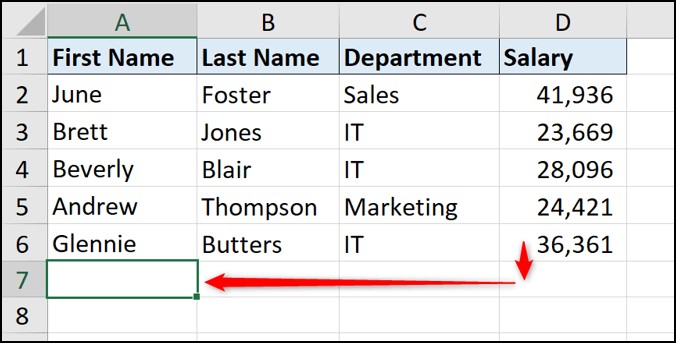
- Split the “Name” column into “First Name” and “Last Name” columns.
- Change the data type of the “Email” column to text.
- Loading Data into Excel:
- After transforming your data, click “Close & Load” to load the data into an Excel worksheet.
- Tips for Using Power Query:
- Plan Your Transformations: Plan your data transformations carefully to ensure you achieve the desired results.
- Use Descriptive Step Names: Use descriptive names for each step in your Power Query query to make it easier to understand and maintain.
- Test Your Queries: Thoroughly test your queries to ensure they work correctly and don’t cause errors.
4.2 Power Pivot: Data Modeling and Analysis
Power Pivot is an in-memory data modeling component for Microsoft Excel. It is used for performing data analysis on large data sets.
-
Enabling Power Pivot:
- Go to File > Options > Add-Ins.
- In the “Manage” dropdown, select “COM Add-ins” and click “Go.”
- Check the box next to “Microsoft Power Pivot for Excel” and click “OK.”
-
Importing Data into Power Pivot:
- Go to the Power Pivot tab and click “Manage.”
- In the Power Pivot window, click “Get External Data” and choose the data source you want to import from.
- Follow the prompts to connect to the data source and select the data you want to import.
-
Creating Relationships between Tables:
- In the Power Pivot window, click “Diagram View.”
- Drag a field from one table to a field in another table to create a relationship between the tables.
-
Writing DAX Formulas:
- DAX (Data Analysis Expressions) is the formula language used in Power Pivot.
- DAX formulas can be used to create calculated columns and measures.
-
Example: Creating a Calculated Measure:
Total Sales := SUM(Sales[Sales Amount])This DAX formula calculates the total sales amount from the “Sales” table.
-
Tips for Using Power Pivot:
- Understand Your Data: Understand your data and how the tables relate to each other.
- Use Descriptive Table and Field Names: Use clear and descriptive table and field names to make your data model easier to understand.
- Optimize Your Data Model: Optimize your data model by removing unnecessary columns and creating relationships between tables.
5. Excel Best Practices and Tips
To master Excel, it’s crucial to adopt best practices and efficient workflows. These tips will help you avoid common pitfalls and maximize your productivity.
5.1 Structuring Your Data Effectively
Properly structuring your data is fundamental to effective analysis and reporting. Here are some best practices for organizing your data:
-
Use a Tabular Format:
- Organize your data in rows and columns, with each column representing a specific attribute and each row representing a unique record.
-
Use Headers:
- Include a header row at the top of your data with clear and descriptive column names.
-
Avoid Empty Rows and Columns:
- Remove any empty rows and columns from your data to prevent errors in calculations and analysis.
-
Use Consistent Data Types:
- Ensure that each column contains data of the same type (e.g., numbers, text, dates).
-
Avoid Merged Cells:
- Avoid using merged cells, as they can cause problems with sorting, filtering, and calculations.
-
Use Tables:
- Convert your data range into a table (Insert > Table) for automatic formatting, filtering, and sorting.
-
Example: Properly Structured Data:
Name Email Date of Birth Sales Amount John Doe [email protected] 1990-05-15 100 Jane Smith [email protected] 1985-12-20 150
5.2 Optimizing Performance in Excel
Optimizing Excel’s performance is essential when working with large datasets or complex calculations. These tips will help you improve the speed and responsiveness of Excel:
- Reduce Formula Complexity:
- Simplify your formulas by breaking them down into smaller, more manageable parts.
- Avoid using volatile functions (e.g., NOW(), TODAY(), RAND()) unnecessarily, as they recalculate every time the worksheet is changed.
- Use Efficient Formulas:
- Use INDEX and MATCH instead of VLOOKUP for faster lookups.
- Use array formulas sparingly, as they can slow down performance.
- Minimize Data:
- Remove unnecessary data from your worksheet.
- Use Power Query to filter and transform data before loading it into Excel.
- Disable Automatic Calculations:
- Set calculation mode to manual (Formulas > Calculation Options > Manual) and recalculate the worksheet only when needed.
- Use Excel Tables:
- Excel tables are optimized for performance and can handle large datasets more efficiently.
- Avoid Excessive Formatting:
- Limit the use of conditional formatting and other formatting options, as they can slow down performance.
- Use the Latest Version of Excel:
- The latest version of Excel includes performance improvements and optimizations.
5.3 Securing and Protecting Your Excel Files
Protecting your Excel files is crucial to prevent unauthorized access and data breaches. These tips will help you secure your files:
- Set a Password:
- Set a password to prevent unauthorized access to your Excel file (File > Info > Protect Workbook > Encrypt with Password).
- Protect Your Worksheets:
- Protect your worksheets to prevent unauthorized changes to data (Review > Protect Sheet).
- Control User Access:
- Control user access to your Excel file by setting permissions on a shared network drive or in a cloud storage service.
- Remove Personal Information:
- Remove personal information from your Excel file before sharing it with others (File > Info > Inspect Document).
- Use Digital Signatures:
- Use digital signatures to verify the authenticity and integrity of your Excel file.
6. Staying Current with Excel Updates and Trends
Excel is constantly evolving with new features and updates. Staying current with these changes is essential for maximizing your productivity and leveraging the latest tools.
6.1 Following Microsoft Excel Blogs and Forums
Following official Microsoft Excel blogs and forums can provide valuable insights into new features, updates, and best practices. Some recommended resources include:
- Microsoft Excel Blog:
- The official Microsoft Excel blog provides updates on new features, tips, and tutorials.
- Microsoft Tech Community:
- The Microsoft Tech Community is a forum where you can ask questions, share knowledge, and connect with other Excel users.
- Excel Subreddit:
- The Excel Subreddit is a community-driven forum where you can discuss Excel topics, ask questions, and share tips and tricks.
6.2 Participating in Excel Training and Workshops
Participating in Excel training and workshops can provide structured learning and hands-on experience with new features and techniques. Look for training opportunities from reputable providers, such as:
-
Microsoft Virtual Academy:
- The Microsoft Virtual Academy offers free online courses on various Excel topics.
-
LinkedIn Learning:
- LinkedIn Learning offers a wide range of Excel courses taught by industry experts.
-
Udemy:
- Udemy offers a variety of Excel courses for all skill levels.
-
LEARNS.EDU.VN:
-
learns.edu.vn connect you with education experts.
6.3 Exploring New Excel Features and Add-Ins
Regularly exploring new Excel features and add-ins can help you discover tools that can improve your productivity and efficiency. Some notable features and add-ins to explore include:
| Feature/Add-In | Description | Benefits |
|---|---|---|
| Power Query | Data transformation and data preparation engine. | Import data from various sources, clean and transform it, and load it into Excel. |
| Power Pivot | In-memory data modeling component for Microsoft Excel. | Perform data analysis on large datasets and create complex data models. |
| Power BI | Business intelligence and data visualization tool. | Create interactive dashboards and reports to visualize and analyze your data. |
| Solver | Optimization tool for solving linear and nonlinear problems. | Find optimal solutions to complex problems, such as resource allocation and scheduling. |
| Analysis ToolPak | Collection of data analysis tools, including ANOVA, regression, and histograms. | Perform statistical analysis and data modeling. |
7. Common Challenges and How to Overcome Them
Learning Excel can present various challenges, especially when progressing to more advanced topics. Recognizing these challenges and having strategies to overcome them is crucial for continuous improvement.
7.1 Dealing with Complex Formulas
Complex formulas can be daunting, but breaking them down into smaller parts and using helper columns can make them more manageable.
-
Challenge: Difficulty understanding and troubleshooting complex formulas.
-
Solution:
- Break Down Formulas: Deconstruct complex formulas into smaller, more understandable parts.
- Use Helper Columns: Create helper columns to perform intermediate calculations and simplify the main formula.
- Use Comments: Add comments to your formulas to explain what each part does.
- Test Your Formulas: Test your formulas with sample data to ensure they produce the correct results.
- Use the Formula Evaluator: Use the Formula Evaluator (Formulas > Evaluate Formula) to step through the calculation process and identify errors.
-
Example:
Instead of using a single complex formula to calculate a weighted average, break it down into smaller formulas in helper columns.
| Value | Weight | Weighted Value |
| —– | —— | ————– |
| 10 | 0.2 | =A2B2 |
| 20 | 0.3 | =A3B3 |
| 30 | 0.5 | =A4*B4 |
| | | Total: |
| | | =SUM(C2:C4) |
7.2 Handling Large Datasets
Large datasets can slow down Excel and make it difficult to analyze data. Using Power Query and Power Pivot can help you handle large datasets more efficiently.
- Challenge: Slow performance and memory issues when working with large datasets.
- Solution:
- Use Power Query: Use Power Query to filter and transform data before loading it into Excel.
- Use Power Pivot: Use Power Pivot to store and analyze large datasets.
- Use Excel Tables: Use Excel tables, as they are optimized for performance.
- Minimize Formulas: Minimize the use of formulas, especially volatile functions.
- Optimize File Size: Save your Excel file in a binary format (.xlsb) to reduce file size.
7.3 Troubleshooting Errors
Errors in Excel can be frustrating, but understanding the different types of errors and how to troubleshoot them can save you time and effort.
-
Challenge: Encountering errors in formulas and data validation.
-
Solution:
- Understand Error Types: Familiarize yourself with common Excel error types, such as #DIV/0!, #NAME?, #VALUE!, and #REF!.
- Use Error Checking: Use Excel’s error checking feature (Formulas > Error Checking) to identify and resolve errors.
- Trace Error Precedents and Dependents: Use the Trace Precedents and Trace Dependents features to understand how errors propagate through your formulas.
- Check Data Validation Rules: Ensure that your data validation rules are set up correctly and that the data being entered is valid.
- Use the IFERROR Function: Use the IFERROR function to handle errors gracefully and prevent them from disrupting your calculations.
-
Example:
Use the IFERROR function to return a default value when a formula results in an error:
=IFERROR(A1/B1, "Error")
7.4 Managing Complex Data Models
Complex data models can be difficult to manage, but using clear naming conventions and documenting your data model can help you stay organized.
- Challenge: Managing complex data models with multiple tables and relationships.
- Solution:
- Use Clear Naming Conventions: Use clear and descriptive names for tables, columns, and relationships.
- Document Your Data Model: Create a data dictionary to document the purpose and structure of each table and column in your data model.
- Use Diagram View: Use the Diagram View in