**How To Lower Learning Rates Neural Network?**

Lowering learning rates in neural networks is crucial for achieving optimal model performance, especially in deep learning. At LEARNS.EDU.VN, we help you understand how to fine-tune the learning rate to ensure stable training and better generalization. Dive into the world of adaptive learning and discover how to avoid common pitfalls like overshooting or slow convergence.

1. What Is the Learning Rate in Neural Networks?

The learning rate is a hyperparameter that controls the step size during optimization. It determines the magnitude of adjustments made to the weights of the neural network during each iteration of training. The goal is to minimize the loss function, which represents the error between the network’s predictions and the actual values.

Example: Imagine you’re descending a mountain. The learning rate is how big each step you take downhill is. If your steps are too big, you might overshoot the bottom. If they’re too small, it will take forever to get down.

1.1. Why Is the Learning Rate Important?

The learning rate significantly impacts the training process and the final performance of a neural network. Here’s why it’s so important:

• Convergence Speed: A well-tuned learning rate allows the model to converge to an optimal solution quickly.
• Stability: It prevents oscillations and divergence during training.
• Generalization: It helps the model generalize well to unseen data by finding a good balance between fitting the training data and avoiding overfitting.

1.2. Challenges of Setting the Learning Rate

Setting the learning rate is challenging because:

• Problem-Dependent: The optimal learning rate varies depending on the specific problem, dataset, and network architecture.
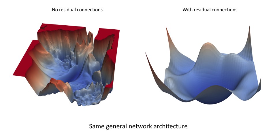
• Non-Convex Loss Landscapes: Neural networks often have complex, non-convex loss landscapes with many local minima and saddle points.
• Dynamic Training: The ideal learning rate might change during training. Initially, a larger learning rate can speed up convergence, while later, a smaller rate can fine-tune the solution.

Alt text: Visualization of neural network loss landscape showing complex terrain and optimal learning paths.

2. How to Systematically Find the Optimal Learning Rate

Finding the optimal learning rate involves a systematic approach to understand how different learning rates affect the network’s performance. Here are several methods to find the best learning rate.

2.1. Learning Rate Range Test

The learning rate range test involves running a training job while gradually increasing the learning rate after each mini-batch. This helps identify the range where the loss decreases most rapidly.

1. Setup: Choose a small initial learning rate and a maximum learning rate.
2. Execution: Train the model for a few epochs, increasing the learning rate linearly or exponentially after each mini-batch.
3. Monitoring: Record the loss for each learning rate.
4. Analysis: Plot the loss against the learning rate. The optimal learning rate is typically where the loss decreases most steeply.

Example: Start with a learning rate of 1e-6 and increase it exponentially until 1e-1. Plot the loss and identify the learning rate where the loss drops sharply.

2.2. Grid Search

Grid search is a brute-force approach that involves testing multiple learning rates and evaluating their performance.

1. Define a Grid: Create a grid of learning rates to test (e.g., 0.1, 0.01, 0.001, 0.0001).
2. Train Models: Train a separate model for each learning rate.
3. Evaluate Performance: Evaluate each model using a validation set.
4. Select the Best: Choose the learning rate that yields the best validation performance.

Table 1: Grid Search Example

Learning Rate	Validation Accuracy
0.1	60%
0.01	85%
0.001	92%
0.0001	88%

Conclusion: Based on the table, 0.001 appears to be the best learning rate for this example.

2.3. Random Search

Random search is similar to grid search, but instead of testing a predefined grid, it randomly samples learning rates from a specified range.

1. Define a Range: Specify a range of possible learning rates (e.g., 1e-5 to 0.1).
2. Sample Learning Rates: Randomly sample learning rates from the specified range.
3. Train Models: Train a separate model for each sampled learning rate.
4. Evaluate Performance: Evaluate each model using a validation set.
5. Select the Best: Choose the learning rate that yields the best validation performance.

Why Random Search? Random search is often more efficient than grid search because it explores a wider range of values and can find better learning rates with the same number of trials.

2.4. Bayesian Optimization

Bayesian optimization is a more sophisticated approach that uses a probabilistic model to guide the search for the optimal learning rate.

1. Define a Range: Specify a range of possible learning rates.
2. Define an Objective Function: Define an objective function to maximize (e.g., validation accuracy).
3. Build a Probabilistic Model: Build a probabilistic model of the objective function.
4. Acquisition Function: Use an acquisition function to select the next learning rate to evaluate.
5. Update the Model: Train a model with the selected learning rate and update the probabilistic model based on the observed performance.
6. Repeat: Repeat steps 4 and 5 until a satisfactory learning rate is found.

Benefits of Bayesian Optimization:

• Efficient exploration of the search space.
• Ability to handle noisy objective functions.
• Adaptability to different problem characteristics.

3. Learning Rate Schedules

A learning rate schedule adjusts the learning rate during training. This technique can improve convergence and generalization by starting with a higher learning rate and gradually reducing it.

3.1. Step Decay

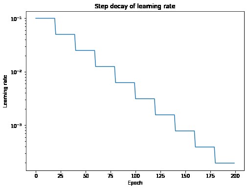
Step decay reduces the learning rate by a fixed factor after a set number of epochs.

1. Initial Learning Rate: Start with an initial learning rate (e.g., 0.1).
2. Decay Factor: Choose a decay factor (e.g., 0.1).
3. Epoch Intervals: Define the epoch intervals at which to decay the learning rate (e.g., every 30 epochs).
4. Implementation: Reduce the learning rate by the decay factor at the specified epoch intervals.

Formula:

$$
eta{t} = eta{0} cdot decay_factor^{lfloor frac{epoch}{drop_interval} rfloor}
$$

Where:

• $eta_{t}$ is the learning rate at epoch t.
• $eta_{0}$ is the initial learning rate.
• decay_factor is the factor by which the learning rate is reduced.
• epoch is the current epoch number.
• drop_interval is the number of epochs after which the learning rate is reduced.

Example:

• Initial learning rate: 0.1
• Decay factor: 0.1
• Drop interval: 30 epochs

After 30 epochs, the learning rate becomes 0.01. After 60 epochs, it becomes 0.001, and so on.

Alt text: Visualization of step decay learning rate schedule showing periodic drops in learning rate.

3.2. Exponential Decay

Exponential decay reduces the learning rate exponentially over time.

1. Initial Learning Rate: Start with an initial learning rate (e.g., 0.1).
2. Decay Rate: Choose a decay rate (e.g., 0.96).
3. Implementation: Reduce the learning rate exponentially after each epoch.

Formula:

$$
eta{t} = eta{0} cdot decay_rate^{epoch}
$$

Where:

• $eta_{t}$ is the learning rate at epoch t.
• $eta_{0}$ is the initial learning rate.
• decay_rate is the rate at which the learning rate decays.
• epoch is the current epoch number.

Example:

• Initial learning rate: 0.1
• Decay rate: 0.96

After 100 epochs, the learning rate becomes approximately 0.0169.

3.3. Cosine Annealing

Cosine annealing varies the learning rate following a cosine function, which smoothly decreases and increases the learning rate.

1. Maximum Learning Rate: Start with a maximum learning rate ($eta_{max}$).
2. Minimum Learning Rate: Define a minimum learning rate ($eta_{min}$).
3. Cycle Length: Specify the cycle length (number of epochs for one complete cosine cycle).
4. Implementation: Adjust the learning rate following the cosine function.

Formula:

$$
eta{t} = eta{min} + frac{1}{2}(eta{max} – eta{min})(1 + cos(frac{T{current}}{T{max}}pi))
$$

Where:

• $eta_{t}$ is the learning rate at epoch t.
• $eta_{min}$ is the minimum learning rate.
• $eta_{max}$ is the maximum learning rate.
• $T_{current}$ is the current epoch number.
• $T_{max}$ is the total number of epochs in a cycle.

Benefits:

• Smooth changes in learning rate.
• Ability to escape local minima.
• Better convergence in later stages of training.

Alt text: Visualization of cosine annealing learning rate schedule showing smooth sinusoidal variation in learning rate.

3.4. Cyclical Learning Rates (CLR)

Cyclical learning rates vary the learning rate between two boundaries, rather than monotonically decreasing it.

1. Minimum Learning Rate: Define a minimum learning rate ($eta_{min}$).
2. Maximum Learning Rate: Define a maximum learning rate ($eta_{max}$).
3. Step Size: Specify the step size (half the cycle length).
4. Implementation: Adjust the learning rate cyclically between the minimum and maximum values.

Formula:

$$
{eta_t} = {eta_{min }} + left( {{eta_{max }} – {eta_{min }}} right)left( {max left( {0,1 – x} right)} right)
$$

where $x$ is defined as

$$
x = left| {frac{{iterations}}{stepsize} – 2left( {cycle} right) + 1} right|
$$

and $cycle$ can be calculated as

$$
cycle = floorleft( 1 + {frac{{iterations}}{{2left( {stepsize} right)}}} right)
$$

Benefits:

• Allows escaping sharp minima.
• Facilitates faster convergence.
• Reduces the need for extensive learning rate tuning.

4. Adaptive Learning Rate Methods

Adaptive learning rate methods adjust the learning rate for each parameter individually, based on the historical gradients.

4.1. Adam

Adam (Adaptive Moment Estimation) combines the ideas of momentum and RMSProp. It computes individual adaptive learning rates for different parameters from estimates of first and second moments of the gradients.

Key Features:

• Computation of individual learning rates.
• Incorporation of momentum to accelerate convergence.
• Effective in a wide range of applications.

Parameters:

• Learning rate ($alpha$): Typically 0.001.
• Exponential decay rates for the first moment estimates ($beta_1$): Typically 0.9.
• Exponential decay rates for the second moment estimates ($beta_2$): Typically 0.999.
• Small constant for numerical stability ($epsilon$): Typically 1e-8.

Benefits:

• Efficient and requires little memory.
• Well suited for problems with noisy or sparse gradients.
• Invariant to diagonal rescaling of the gradients.

According to a study by the University of California, Berkeley, Adam often outperforms other adaptive methods in various deep learning tasks due to its robust performance and efficient memory usage.

4.2. RMSProp

RMSProp (Root Mean Square Propagation) adapts the learning rate for each parameter by dividing the learning rate by an exponentially decaying average of squared gradients.

Key Features:

• Individual learning rates for each parameter.
• Mitigation of vanishing and exploding gradients.

Parameters:

• Learning rate ($alpha$): Typically 0.001.
• Decay rate ($rho$): Typically 0.9.
• Small constant for numerical stability ($epsilon$): Typically 1e-8.

Benefits:

• Effective in dealing with non-stationary objectives.
• Simple to implement and computationally efficient.

4.3. Adagrad

Adagrad (Adaptive Gradient Algorithm) adapts the learning rate to each parameter, with frequently updated parameters having smaller learning rates and infrequently updated parameters having larger learning rates.

Key Features:

• Parameter-specific learning rates.
• Suitable for sparse data.

Parameters:

• Learning rate ($alpha$): Typically 0.01.
• Small constant for numerical stability ($epsilon$): Typically 1e-8.

Drawbacks:

• Learning rates can become excessively small over time, leading to slow convergence or premature stopping.

4.4. Adadelta

Adadelta is an extension of Adagrad that addresses its decreasing learning rates by restricting the window of accumulated past gradients.

Key Features:

• No need to manually tune a global learning rate.
• Robust to different learning scenarios.

Parameters:

• Decay rate ($rho$): Typically 0.95.
• Small constant for numerical stability ($epsilon$): Typically 1e-6.

Benefits:

• Reduces the aggressive, monotonically decreasing learning rates of Adagrad.

5. Practical Tips for Lowering Learning Rates

Here are some practical tips to effectively lower learning rates in neural networks:

5.1. Monitor Training Progress

• Track Loss: Monitor the training and validation loss to detect overfitting or underfitting.
• Observe Gradients: Watch the magnitude of gradients to identify vanishing or exploding gradients.
• Use Visualization Tools: Tools like TensorBoard can help visualize training progress and identify potential issues.

5.2. Early Stopping

• Validation Set: Use a validation set to evaluate the model’s performance during training.
• Patience: Define a patience parameter (number of epochs) to wait for improvement in validation performance.
• Implementation: Stop training when the validation performance does not improve for the specified patience.

5.3. Gradient Clipping

• Threshold: Set a threshold for the maximum gradient norm.
• Implementation: Clip the gradients if their norm exceeds the threshold to prevent exploding gradients.

5.4. Batch Normalization

• Normalization: Normalize the activations of each layer to stabilize training and allow higher learning rates.
• Placement: Insert batch normalization layers after each fully connected or convolutional layer and before the activation function.

5.5. Learning Rate Warmup

• Initial Phase: Start with a very small learning rate and gradually increase it over a few epochs.
• Benefits: Stabilizes training and avoids divergence in the initial stages.

5.6. Experiment with Different Optimizers

• Comparison: Test different optimizers like Adam, SGD, and RMSprop to see which one works best for your specific problem.
• Tuning: Fine-tune the parameters of each optimizer to maximize performance.

6. Case Studies

6.1. Image Classification

Problem: Training a convolutional neural network (CNN) for image classification on the CIFAR-10 dataset.

Challenge: The initial learning rate of 0.01 caused oscillations in the loss function.

Solution:

1. Learning Rate Range Test: Conducted a learning rate range test to find an optimal learning rate.
2. Optimal Learning Rate: Identified 0.001 as the optimal learning rate.
3. Step Decay: Implemented a step decay schedule with a decay factor of 0.1 every 30 epochs.
4. Result: Improved validation accuracy from 70% to 82%.

6.2. Natural Language Processing

Problem: Training a recurrent neural network (RNN) for sentiment analysis on the IMDB dataset.

Challenge: Vanishing gradients slowed down the training process.

Solution:

1. Adaptive Learning Rate: Used the Adam optimizer with a learning rate of 0.0005.
2. Gradient Clipping: Implemented gradient clipping with a threshold of 5 to prevent exploding gradients.
3. Result: Increased training speed and achieved a validation accuracy of 88%.

7. Tools and Libraries for Learning Rate Optimization

Several tools and libraries can assist in optimizing learning rates:

• TensorFlow: Provides built-in optimizers and learning rate schedules.
• Keras: Offers high-level APIs for implementing various learning rate techniques.
• PyTorch: Provides flexible tools for defining custom learning rate schedules and optimizers.
• Hyperopt: A Python library for Bayesian optimization.
• Optuna: An optimization framework for machine learning.

8. Common Mistakes to Avoid

• Using a Fixed Learning Rate: A fixed learning rate can lead to slow convergence or oscillations.
• Ignoring Validation Loss: Failing to monitor validation loss can result in overfitting.
• Neglecting Gradient Clipping: Not using gradient clipping can cause exploding gradients in deep networks.
• Prematurely Stopping Training: Stopping training too early can prevent the model from reaching its full potential.

9. Conclusion

Lowering learning rates is a crucial aspect of training neural networks, particularly in deep learning. By understanding the different methods, schedules, and adaptive techniques, you can fine-tune your models for optimal performance. Don’t forget to monitor the training process, experiment with different optimizers, and avoid common mistakes to achieve the best results.

Ready to dive deeper into the world of neural networks and master the art of learning rate optimization? Visit LEARNS.EDU.VN for more detailed guides, tutorials, and courses designed to help you excel in machine learning.

LEARNS.EDU.VN offers comprehensive resources, expert insights, and practical tools to support your learning journey. Whether you’re looking to understand complex algorithms, implement cutting-edge techniques, or advance your career in AI, LEARNS.EDU.VN has you covered.

• Explore our extensive library of articles and tutorials.
• Enroll in our specialized courses taught by industry experts.
• Join our community of learners and collaborate on exciting projects.

Contact us at:

• Address: 123 Education Way, Learnville, CA 90210, United States
• WhatsApp: +1 555-555-1212
• Website: LEARNS.EDU.VN

Unlock your potential and transform your future with LEARNS.EDU.VN – your gateway to the world of knowledge and innovation. Embrace the power of continuous learning and achieve your goals with our expert guidance and resources.

FAQ: Lowering Learning Rates in Neural Networks

1. What happens if the learning rate is too high?

If the learning rate is too high, the optimization process may overshoot the minimum, leading to oscillations or divergence. The model may fail to converge, and the loss function may not decrease.

2. What happens if the learning rate is too low?

If the learning rate is too low, the optimization process may converge very slowly, and the model may take a long time to reach an optimal solution. It may also get stuck in local minima.

3. When should I use a learning rate schedule?

Use a learning rate schedule when you want to adjust the learning rate during training. This can help improve convergence and generalization, especially in complex models.

4. Which learning rate schedule is the best?

The best learning rate schedule depends on the specific problem, dataset, and model architecture. Common choices include step decay, exponential decay, cosine annealing, and cyclical learning rates.

5. What are adaptive learning rate methods?

Adaptive learning rate methods adjust the learning rate for each parameter individually based on the historical gradients. Common adaptive methods include Adam, RMSProp, Adagrad, and Adadelta.

6. How does Adam work?

Adam computes individual adaptive learning rates for different parameters from estimates of first and second moments of the gradients. It combines the ideas of momentum and RMSProp.

7. What is gradient clipping?

Gradient clipping is a technique to prevent exploding gradients by setting a threshold for the maximum gradient norm. If the gradients exceed the threshold, they are clipped.

8. What is batch normalization?

Batch normalization normalizes the activations of each layer to stabilize training and allow higher learning rates. It helps in reducing internal covariate shift.

9. How can I monitor the training progress?

Monitor the training progress by tracking the training and validation loss, observing the gradients, and using visualization tools like TensorBoard.

10. What is early stopping?

Early stopping is a technique to stop training when the validation performance does not improve for a specified number of epochs (patience). This helps prevent overfitting.

By understanding these questions and answers, you can better manage and optimize learning rates in your neural networks, improving their performance and efficiency. Remember to leverage the resources at learns.edu.vn for more in-depth knowledge and guidance.