What Is Accuracy In Machine Learning And Why Does It Matter?

Accuracy is a cornerstone metric in machine learning, but its implications and interpretations vary widely depending on the context. Understanding accuracy, its nuances, and its alternatives is critical for building reliable and effective models. Let’s explore what accuracy means in machine learning and why it is important. Discover comprehensive resources and expert guidance at LEARNS.EDU.VN.

1. Understanding Accuracy in Machine Learning

Accuracy in machine learning is the measure of how well a model correctly predicts outcomes. It is calculated as the ratio of correct predictions to the total number of predictions made. In simpler terms, it tells you how often the model is right.

1.1. Definition of Accuracy

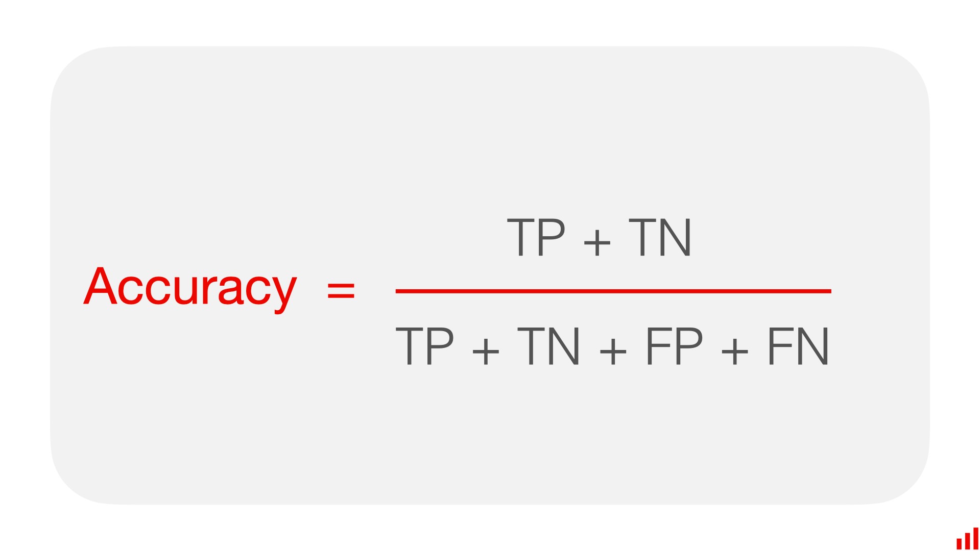
Accuracy is a fundamental metric in machine learning that indicates the proportion of correct predictions made by a model out of the total predictions. It serves as an initial gauge of a model’s overall effectiveness. The formula to calculate accuracy is straightforward:

Accuracy = (Number of Correct Predictions) / (Total Number of Predictions)

This metric is expressed as a decimal or a percentage, where a higher value indicates better performance. For example, an accuracy of 0.95 (or 95%) means that the model correctly predicts the outcome 95% of the time.

1.2. How to Calculate Accuracy

Calculating accuracy is straightforward. For instance, consider a scenario where a machine learning model makes 100 predictions, and 80 of those predictions are correct. The accuracy is calculated as follows:

Accuracy = 80 / 100 = 0.8 or 80%

This indicates that the model correctly predicts the outcome 80% of the time.

1.3. The Importance of Accuracy as a Metric

Accuracy is important because it provides a high-level overview of the model’s performance. Here’s why it matters:

Intuitive Understanding: Accuracy is easy to understand and explain, making it a good starting point for evaluating model performance.
Overall Performance Indicator: It gives a general sense of how well the model is performing across all classes.
Benchmarking: Accuracy can be used as a benchmark to compare different models or different versions of the same model.

1.4. Real-World Examples Where Accuracy Is Crucial

Accuracy is particularly valuable in scenarios where balanced class distribution exists and the costs of false positives and false negatives are similar. Here are some examples:

Image Recognition: In applications such as identifying objects in images (e.g., cats versus dogs), accuracy helps ensure that the model correctly classifies the majority of images.
Sentiment Analysis: When determining the sentiment of text data, accuracy measures how often the model correctly identifies positive, negative, or neutral sentiments.

2. The Accuracy Paradox: When Accuracy Fails

The accuracy paradox arises when a model achieves high accuracy, but it is misleading due to imbalanced datasets. This section explores this paradox and its implications.

2.1. What is the Accuracy Paradox?

The accuracy paradox occurs when a model exhibits high accuracy scores, yet fails to provide practical utility. This often happens when dealing with imbalanced datasets, where one class significantly outweighs the other. In such cases, a model can achieve high accuracy by simply predicting the majority class, rendering it ineffective for identifying the minority class, which is usually of greater interest.

2.2. Imbalanced Datasets and Misleading Accuracy

In imbalanced datasets, the distribution of classes is heavily skewed. For example, in a dataset for fraud detection, fraudulent transactions may only account for 1% of the total transactions. A model that always predicts “no fraud” can achieve 99% accuracy, which seems impressive but is practically useless because it fails to detect any fraudulent transactions.

2.3. Examples of the Accuracy Paradox in Real-World Scenarios

Here are a few real-world examples where the accuracy paradox can be problematic:

Medical Diagnosis: In detecting rare diseases, a model that predicts “no disease” for all patients may achieve high accuracy if the disease prevalence is low, but it will fail to identify actual cases.
Fraud Detection: As mentioned earlier, in fraud detection, a model that always predicts “no fraud” can have high accuracy but fail to detect any fraudulent activities.
Predictive Maintenance: In predicting equipment failures, a model that rarely predicts failures can achieve high accuracy but fail to identify machines at risk of breakdown.

2.4. How to Identify the Accuracy Paradox

To identify the accuracy paradox, consider the following steps:

Examine Class Distribution: Check the distribution of classes in the dataset. If there is a significant imbalance, be cautious about relying solely on accuracy.
Evaluate Other Metrics: Use additional metrics such as precision, recall, F1-score, and AUC-ROC to get a more comprehensive view of the model’s performance.
Analyze Confusion Matrix: Review the confusion matrix to understand how the model is performing on each class. This will reveal if the model is simply predicting the majority class.
Assess Business Impact: Consider the practical implications of the model’s predictions. Does the model provide valuable insights, or is it simply confirming the status quo?

3. Precision and Recall: Better Metrics for Imbalanced Datasets

Precision and recall are two critical metrics that provide a more granular evaluation of a model’s performance, especially in scenarios with imbalanced datasets.

3.1. Defining Precision and Recall

Precision: Precision measures the accuracy of the positive predictions made by the model. It is the ratio of true positives (correctly predicted positive instances) to the total number of instances predicted as positive (both true positives and false positives).

Precision = True Positives / (True Positives + False Positives)
Recall: Recall measures the model’s ability to identify all relevant instances of the positive class. It is the ratio of true positives to the total number of actual positive instances (both true positives and false negatives).

Recall = True Positives / (True Positives + False Negatives)

3.2. How Precision and Recall Work

Precision and recall provide insight into different aspects of a model’s performance. High precision means the model is good at avoiding false positives, while high recall means the model is good at avoiding false negatives. The choice between prioritizing precision or recall depends on the specific problem and the associated costs of different types of errors.

3.3. The Trade-off Between Precision and Recall

There is often a trade-off between precision and recall. Increasing one metric may decrease the other. For example, to increase recall, a model might predict more instances as positive, which could lead to more false positives, thereby reducing precision. Conversely, to increase precision, a model might be more selective in its positive predictions, which could result in more false negatives, thereby reducing recall.

3.4. Visual Examples Demonstrating Precision and Recall

Consider a scenario where a model is used to detect defective products in a manufacturing plant.

High Precision: If the model has high precision, it means that when it identifies a product as defective, it is likely to be truly defective. This is important to avoid unnecessary discarding of good products.
High Recall: If the model has high recall, it means that it identifies most of the defective products. This is crucial to ensure that defective products do not reach the customers.

3.5. When to Prioritize Precision vs. Recall

The decision to prioritize precision or recall depends on the specific use case and the costs associated with false positives and false negatives.

Prioritize Precision When:
- False positives are costly.
- The goal is to minimize incorrect positive predictions.
- Example: Spam filtering. It is better to let a few spam emails through (false negatives) than to incorrectly classify important emails as spam (false positives).
Prioritize Recall When:
- False negatives are costly.
- The goal is to minimize missed positive instances.
- Example: Medical diagnosis. It is better to have a few false alarms (false positives) than to miss identifying a serious illness (false negatives).

4. F1-Score: Balancing Precision and Recall

The F1-score is a single metric that balances both precision and recall, providing a more comprehensive measure of a model’s performance, especially in imbalanced datasets.

4.1. Definition of F1-Score

The F1-score is the harmonic mean of precision and recall. It provides a balanced measure of a model’s performance, considering both its ability to avoid false positives and false negatives. The formula for the F1-score is:

F1-Score = 2 * (Precision * Recall) / (Precision + Recall)

4.2. How to Calculate the F1-Score

To calculate the F1-score, you need the values of precision and recall. For example, if a model has a precision of 0.8 and a recall of 0.9, the F1-score is calculated as follows:

F1-Score = 2 * (0.8 * 0.9) / (0.8 + 0.9) = 2 * 0.72 / 1.7 = 0.847

This indicates that the model has a balanced performance, with both precision and recall contributing significantly to the score.

4.3. Advantages of Using the F1-Score

The F1-score offers several advantages:

Balanced Metric: It balances precision and recall, making it suitable for imbalanced datasets where accuracy can be misleading.
Single Metric: It provides a single, easy-to-interpret metric that summarizes the model’s overall performance.
Useful for Trade-off Analysis: It helps in making informed decisions when there is a trade-off between precision and recall.

4.4. Scenarios Where F1-Score is Most Useful

The F1-score is particularly useful in scenarios where both precision and recall are important, and there is a need to balance the trade-off between them. Examples include:

Spam Detection: Balancing the need to minimize false positives (important emails classified as spam) and false negatives (spam emails reaching the inbox).
Medical Diagnosis: Balancing the need to minimize false positives (unnecessary treatments) and false negatives (missed diagnoses).
Fraud Detection: Balancing the need to minimize false positives (blocking legitimate transactions) and false negatives (undetected fraudulent activities).

4.5. Interpreting F1-Score Values

The F1-score ranges from 0 to 1, with higher values indicating better performance. Here is a general guideline for interpreting F1-score values:

F1-Score > 0.8: Indicates excellent performance, with both precision and recall being high.
F1-Score between 0.6 and 0.8: Indicates good performance, with a reasonable balance between precision and recall.
F1-Score between 0.4 and 0.6: Indicates moderate performance, with potential areas for improvement in either precision or recall.
F1-Score < 0.4: Indicates poor performance, requiring significant improvements in both precision and recall.

5. Other Important Metrics to Consider

While accuracy, precision, recall, and F1-score are essential metrics, other metrics provide additional insights into a model’s performance.

5.1. Area Under the ROC Curve (AUC-ROC)

AUC-ROC is a metric that measures the ability of a model to distinguish between positive and negative classes across different threshold settings.

Definition: The ROC (Receiver Operating Characteristic) curve plots the true positive rate (recall) against the false positive rate at various threshold settings. AUC represents the area under this curve.
How it Works: AUC-ROC provides a single value that summarizes the model’s performance across all possible classification thresholds.
Advantages: It is threshold-invariant, meaning it is not affected by the choice of a specific threshold. It is also useful for imbalanced datasets.
Interpretation: AUC values range from 0 to 1. An AUC of 0.5 indicates that the model performs no better than random chance, while an AUC of 1 indicates perfect discrimination between classes. Generally, an AUC above 0.7 is considered good.

5.2. Specificity and Sensitivity

Specificity and sensitivity provide insights into a model’s ability to correctly identify negative and positive cases, respectively.

Specificity: Specificity (also known as the true negative rate) measures the proportion of actual negatives that are correctly identified by the model. It is calculated as:

Specificity = True Negatives / (True Negatives + False Positives)
Sensitivity: Sensitivity (also known as recall or the true positive rate) measures the proportion of actual positives that are correctly identified by the model. It is calculated as:

Sensitivity = True Positives / (True Positives + False Negatives)
Usefulness: Specificity and sensitivity are particularly useful in medical diagnostics and other applications where correctly identifying both positive and negative cases is critical.

5.3. Confusion Matrix: A Detailed Breakdown

A confusion matrix provides a detailed breakdown of a model’s performance by showing the counts of true positives, false positives, true negatives, and false negatives.

Definition: A confusion matrix is a table that summarizes the results of a classification model by displaying the counts of correct and incorrect predictions for each class.
Components:
- True Positives (TP): Instances correctly predicted as positive.
- False Positives (FP): Instances incorrectly predicted as positive.
- True Negatives (TN): Instances correctly predicted as negative.
- False Negatives (FN): Instances incorrectly predicted as negative.
Usefulness: The confusion matrix provides a comprehensive view of the model’s performance, allowing you to identify specific areas of strength and weakness. It is essential for understanding the types of errors the model is making and for making informed decisions about model improvement.

5.4. Log Loss

Logarithmic loss (also known as log loss or cross-entropy loss) evaluates the performance of a classification model by quantifying the uncertainty of its predictions.

Definition: Log loss measures the accuracy of probabilities predicted by a classification model. It penalizes incorrect predictions more heavily as the predicted probability diverges from the actual label.
Formula: The log loss is calculated as:

Log Loss = – (1/N) * Σ [y * log(p) + (1 – y) * log(1 – p)]

where:
- N is the number of observations.
- y is the actual label (0 or 1).
- p is the predicted probability of the observation being positive.
Interpretation: Log loss values range from 0 to infinity. Lower log loss values indicate better performance, as they reflect more accurate probability predictions. A perfect model has a log loss of 0.

5.5. Cohen’s Kappa

Cohen’s Kappa measures the agreement between predicted and actual labels, accounting for the possibility of agreement occurring by chance.

Definition: Cohen’s Kappa is a statistical measure that assesses the level of agreement between two raters (or, in this case, a model’s predictions and actual labels) while correcting for agreement that could occur randomly.
Formula: Cohen’s Kappa is calculated as:

Kappa = (Po – Pe) / (1 – Pe)

where:
- Po is the observed agreement (accuracy).
- Pe is the expected agreement due to chance.
Interpretation:
- Kappa values range from -1 to 1:
  - 1 indicates perfect agreement.
  - 0 indicates agreement equivalent to chance.
  - -1 indicates perfect disagreement.
- Generally, Kappa values are interpreted as follows:
  - < 0: Poor agreement
  - 0.0 – 0.20: Slight agreement
  - 0.21 – 0.40: Fair agreement
  - 0.41 – 0.60: Moderate agreement
  - 0.61 – 0.80: Substantial agreement
  - 0.81 – 1.0: Almost perfect agreement

6. Practical Considerations for Choosing Metrics

Selecting the right metrics is crucial for accurately evaluating a machine learning model. Here are some practical considerations to keep in mind.

6.1. Understanding Business Objectives

Aligning metrics with business objectives ensures that the model’s performance directly contributes to achieving business goals.

Identify Key Objectives: Clearly define what the business aims to achieve with the model. For example, is the goal to minimize fraud losses, improve customer satisfaction, or reduce operational costs?
Translate Objectives into Metrics: Convert these objectives into measurable metrics. For instance, minimizing fraud losses can be translated into maximizing precision and recall for fraud detection.
Prioritize Metrics: Determine which metrics are most critical for achieving the business objectives. This will guide the selection of metrics for model evaluation and optimization.

6.2. Cost-Sensitive Evaluation

Cost-sensitive evaluation involves assigning costs to different types of errors, allowing for a more nuanced assessment of a model’s performance.

Assign Costs to Errors: Determine the costs associated with false positives and false negatives. For example, the cost of a false negative in medical diagnosis (missing a disease) may be much higher than the cost of a false positive (unnecessary treatment).
Use Cost-Sensitive Metrics: Employ metrics that take these costs into account, such as cost-sensitive accuracy or expected loss.
Optimize for Cost: Optimize the model to minimize the total cost of errors, rather than simply maximizing accuracy or F1-score.

6.3. Segment-Specific Evaluation

Segment-specific evaluation involves evaluating a model’s performance on different segments of the data to identify areas where the model may be underperforming.

Identify Data Segments: Divide the data into meaningful segments based on factors such as demographics, behavior, or geography.
Evaluate Performance on Each Segment: Calculate metrics separately for each segment to identify differences in performance.
Address Underperforming Segments: Develop strategies to improve performance on segments where the model is underperforming. This may involve collecting more data for those segments, tuning the model parameters, or using different models for different segments.

6.4. The Importance of a Baseline Model

A baseline model provides a benchmark against which to compare the performance of more complex models.

Establish a Simple Model: Create a simple model that can serve as a baseline. This could be a model that always predicts the majority class or a simple linear model.
Evaluate Baseline Performance: Calculate metrics for the baseline model to establish a benchmark.
Compare Complex Models: Compare the performance of more complex models to the baseline to determine if they provide a meaningful improvement. If a complex model does not significantly outperform the baseline, it may not be worth the additional complexity.

6.5. Visualizing Metrics for Better Understanding

Visualizing metrics can help in understanding a model’s performance and identifying areas for improvement.

Create Visualizations: Use visualizations such as ROC curves, precision-recall curves, and confusion matrices to display the model’s performance.
Analyze Visualizations: Analyze the visualizations to identify patterns and trends in the model’s performance. For example, a ROC curve that is close to the diagonal line indicates poor performance, while a curve that is close to the top-left corner indicates excellent performance.
Communicate Results: Use visualizations to communicate the model’s performance to stakeholders in a clear and understandable way.

7. Improving Model Accuracy

Improving model accuracy involves a combination of strategies to enhance the model’s ability to make correct predictions.

7.1. Feature Engineering and Selection

Feature engineering and selection involve creating new features from existing ones and selecting the most relevant features to improve model performance.

Feature Engineering: Create new features by combining or transforming existing features. For example, you might create a new feature by calculating the ratio of two existing features or by applying a mathematical function to a feature.
Feature Selection: Select the most relevant features for the model. This can be done using techniques such as univariate selection, recursive feature elimination, or feature importance from tree-based models.
Benefits: Feature engineering and selection can improve model accuracy by providing the model with more informative and relevant features.

7.2. Data Preprocessing Techniques

Data preprocessing techniques involve cleaning and transforming the data to improve its quality and suitability for modeling.

Handling Missing Values: Impute missing values using techniques such as mean imputation, median imputation, or model-based imputation.
Encoding Categorical Variables: Convert categorical variables into numerical form using techniques such as one-hot encoding or label encoding.
Scaling Numerical Variables: Scale numerical variables to a similar range using techniques such as min-max scaling or standardization.
Benefits: Data preprocessing can improve model accuracy by ensuring that the data is clean, consistent, and suitable for modeling.

7.3. Model Selection and Hyperparameter Tuning

Model selection and hyperparameter tuning involve choosing the best model for the data and optimizing its parameters to achieve the best performance.

Model Selection: Evaluate different types of models to determine which one performs best on the data. Consider factors such as the type of problem, the size of the dataset, and the interpretability of the model.
Hyperparameter Tuning: Optimize the hyperparameters of the chosen model using techniques such as grid search, random search, or Bayesian optimization.
Benefits: Model selection and hyperparameter tuning can improve model accuracy by identifying the best model and optimizing its parameters for the data.

7.4. Addressing Overfitting and Underfitting

Overfitting and underfitting are common problems in machine learning that can negatively impact model accuracy.

Overfitting: Overfitting occurs when a model learns the training data too well and performs poorly on new, unseen data.
- Techniques to Address Overfitting:
  - Use more data.
  - Simplify the model (e.g., reduce the number of features or the complexity of the model).
  - Apply regularization techniques (e.g., L1 or L2 regularization).
  - Use dropout in neural networks.
Underfitting: Underfitting occurs when a model is too simple to capture the underlying patterns in the data and performs poorly on both the training and test data.
- Techniques to Address Underfitting:
  - Use a more complex model.
  - Add more features.
  - Reduce regularization.
Benefits: Addressing overfitting and underfitting can improve model accuracy by ensuring that the model generalizes well to new, unseen data.

7.5. Ensemble Methods

Ensemble methods involve combining multiple models to improve overall performance.

Techniques:
- Bagging: Train multiple models on different subsets of the training data and combine their predictions.
- Boosting: Train models sequentially, with each model focusing on correcting the errors made by the previous models.
- Stacking: Combine the predictions of multiple models using another model (a meta-learner).
Benefits: Ensemble methods can improve model accuracy by reducing variance and bias and by combining the strengths of multiple models.

8. Tools for Measuring and Improving Accuracy

Several tools can help in measuring and improving the accuracy of machine learning models.

8.1. Scikit-Learn

Scikit-Learn is a popular Python library that provides a wide range of tools for machine learning, including functions for measuring accuracy and other metrics.

Metrics Functions: Scikit-Learn provides functions for calculating accuracy, precision, recall, F1-score, AUC-ROC, and other metrics.
Model Evaluation Tools: Scikit-Learn provides tools for cross-validation, hyperparameter tuning, and model selection.

Example:

from sklearn.metrics import accuracy_score, classification_report
y_true = [0, 1, 0, 1]
y_pred = [0, 1, 1, 0]
accuracy = accuracy_score(y_true, y_pred)
report = classification_report(y_true, y_pred)
print("Accuracy:", accuracy)
print("Classification Report:n", report)

8.2. TensorFlow and Keras

TensorFlow and Keras are powerful deep learning frameworks that provide tools for building and evaluating neural networks.

Metrics: TensorFlow and Keras provide metrics for measuring accuracy, precision, recall, and other performance indicators.
Model Evaluation: These frameworks allow for detailed model evaluation and provide callbacks for monitoring training progress.

Example (Keras):

import tensorflow as tf
model = tf.keras.Sequential([
    tf.keras.layers.Dense(10, activation='relu', input_shape=(784,)),
    tf.keras.layers.Dense(1, activation='sigmoid')
])
model.compile(optimizer='adam',
              loss='binary_crossentropy',
              metrics=['accuracy'])
model.fit(x_train, y_train, epochs=10, validation_data=(x_val, y_val))

8.3. MLflow

MLflow is an open-source platform for managing the end-to-end machine learning lifecycle, including tracking metrics and experiments.

Experiment Tracking: MLflow allows you to track metrics, parameters, and artifacts for each experiment.
Model Management: MLflow provides tools for managing and deploying models.

Example:

import mlflow
with mlflow.start_run():
    # Log parameters
    mlflow.log_param("learning_rate", 0.01)
    # Train your model here
    # Log metrics
    mlflow.log_metric("accuracy", 0.85)

8.4. Evidently AI

Evidently AI is an open-source Python library that helps evaluate, test, and monitor machine learning models in production.

Comprehensive Reporting: Evidently AI provides detailed reports on model performance, including metrics such as accuracy, precision, recall, and F1-score.
Data Drift Detection: Evidently AI can detect data drift, which can impact model accuracy.
Easy Integration: Evidently AI can be easily integrated into existing machine learning pipelines.

9. Ethical Considerations of Accuracy

Ethical considerations are essential when evaluating and improving the accuracy of machine learning models.

9.1. Bias in Data and Models

Bias in data and models can lead to unfair or discriminatory outcomes, even if the model has high accuracy.

Sources of Bias: Bias can arise from various sources, including biased data, biased algorithms, and biased human decisions.
Impact of Bias: Bias can result in certain groups being unfairly disadvantaged or discriminated against by the model.
Mitigating Bias:
- Collect diverse and representative data.
- Use techniques such as re-weighting or resampling to balance the data.
- Evaluate the model’s performance on different demographic groups.
- Use fairness-aware algorithms that explicitly aim to reduce bias.

9.2. Transparency and Explainability

Transparency and explainability are essential for building trust in machine learning models and for ensuring that they are used ethically.

Importance of Transparency: Transparency allows stakeholders to understand how the model works and what factors it is using to make predictions.
Explainable AI (XAI): Use techniques such as SHAP values, LIME, or interpretable models to explain the model’s decisions.
Benefits: Transparency and explainability can help identify and mitigate bias, build trust in the model, and ensure that it is used ethically.

9.3. Privacy Concerns

Privacy concerns are important when dealing with sensitive data, such as personal information or medical records.

Data Anonymization: Anonymize data to protect individuals’ privacy.
Differential Privacy: Use techniques such as differential privacy to add noise to the data and protect privacy.
Compliance with Regulations: Comply with relevant privacy regulations, such as GDPR or CCPA.

9.4. Accountability and Responsibility

Accountability and responsibility are essential for ensuring that machine learning models are used ethically and responsibly.

Define Roles and Responsibilities: Clearly define roles and responsibilities for the development, deployment, and monitoring of machine learning models.
Establish Oversight Mechanisms: Establish mechanisms for oversight and accountability, such as ethics review boards or data governance committees.
Monitor and Audit Models: Regularly monitor and audit models to ensure that they are performing as expected and are not causing harm.

10. The Future of Accuracy Metrics

The future of accuracy metrics involves developing new and more sophisticated ways to evaluate the performance of machine learning models.

10.1. Contextual Accuracy

Contextual accuracy takes into account the specific context in which the model is being used.

Definition: Contextual accuracy considers factors such as the cost of errors, the business objectives, and the ethical considerations.
Benefits: Contextual accuracy provides a more nuanced and relevant measure of model performance.
Example: In medical diagnosis, contextual accuracy might consider the prevalence of the disease, the cost of false positives and false negatives, and the impact on patient outcomes.

10.2. Adaptive Metrics

Adaptive metrics adjust their behavior based on the performance of the model.

Definition: Adaptive metrics dynamically adjust their parameters or weights based on the model’s performance on different segments of the data or at different points in time.
Benefits: Adaptive metrics can provide a more accurate and relevant measure of model performance in dynamic and changing environments.
Example: An adaptive metric might increase the weight given to segments of the data where the model is underperforming or adjust the threshold for classification based on the current cost of errors.

10.3. Multi-Dimensional Evaluation

Multi-dimensional evaluation involves evaluating the model’s performance along multiple dimensions, such as accuracy, fairness, transparency, and privacy.

Benefits: Multi-dimensional evaluation provides a more holistic and comprehensive view of model performance.
Example: A multi-dimensional evaluation might consider the model’s accuracy, its fairness across different demographic groups, its transparency in terms of explainability, and its compliance with privacy regulations.

10.4. Human-Centered Metrics

Human-centered metrics focus on the impact of the model on human users and stakeholders.

Benefits: Human-centered metrics can help ensure that machine learning models are used in a way that is beneficial and ethical.
Example: Human-centered metrics might measure the impact of the model on user satisfaction, trust, or well-being.

10.5. Integrated Evaluation Frameworks

Integrated evaluation frameworks combine multiple metrics and techniques into a comprehensive evaluation process.

Benefits: Integrated evaluation frameworks provide a more robust and reliable assessment of model performance.
Example: An integrated evaluation framework might include steps for data preprocessing, feature engineering, model selection, hyperparameter tuning, bias detection and mitigation, transparency and explainability, and human-centered evaluation.

FAQ Section

Q1: What Is Accuracy In Machine Learning?

Accuracy is a metric that measures how often a machine learning model correctly predicts the outcome. It is calculated as the ratio of correct predictions to the total number of predictions.

Q2: Why is accuracy important?

Accuracy provides a high-level overview of the model’s performance and is easy to understand and explain. It is also useful for benchmarking different models.

Q3: What is the accuracy paradox?

The accuracy paradox occurs when a model achieves high accuracy but is misleading due to imbalanced datasets. In such cases, the model may simply be predicting the majority class.

Q4: How do precision and recall help in imbalanced datasets?

Precision measures the accuracy of positive predictions, while recall measures the model’s ability to identify all relevant instances of the positive class. These metrics provide a more granular evaluation of the model’s performance in imbalanced datasets.

Q5: What is the F1-score?

The F1-score is the harmonic mean of precision and recall. It provides a balanced measure of a model’s performance, considering both its ability to avoid false positives and false negatives.

Q6: When should I prioritize precision over recall?

Prioritize precision when false positives are costly and the goal is to minimize incorrect positive predictions.

Q7: When should I prioritize recall over precision?

Prioritize recall when false negatives are costly and the goal is to minimize missed positive instances.

Q8: What is AUC-ROC?

AUC-ROC (Area Under the ROC Curve) is a metric that measures the ability of a model to distinguish between positive and negative classes across different threshold settings.

Q9: How can I improve the accuracy of my machine learning model?

You can improve accuracy through feature engineering and selection, data preprocessing, model selection and hyperparameter tuning, addressing overfitting and underfitting, and using ensemble methods.

Q10: What are some ethical considerations when evaluating accuracy?

Ethical considerations include addressing bias in data and models, ensuring transparency and explainability, protecting privacy, and ensuring accountability and responsibility.

Conclusion

Understanding “what is accuracy in machine learning” is fundamental, but it is equally crucial to recognize its limitations and explore alternative metrics like precision, recall, and F1-score. By considering these metrics in conjunction with business objectives and ethical considerations, you can build reliable and effective models that deliver meaningful results.

Ready to dive deeper into the world of machine learning? Visit LEARNS.EDU.VN today to explore our extensive resources, expert tutorials, and comprehensive courses designed to help you master the skills you need to succeed. Whether you are looking to understand complex concepts, learn new techniques, or advance your career, LEARNS.EDU.VN is your trusted partner in education.

Address: 123 Education Way, Learnville, CA 90210, United States
WhatsApp: +1 555-555-1212
Website: LEARNS.EDU.VN

Explore, learn, and grow with learns.edu.vn. Your journey to educational excellence starts here.