What Is PCA in Machine Learning and How Does It Work?

Principal Component Analysis (PCA) in machine learning is a powerful technique for dimensionality reduction and feature extraction, and you can master it with ease at LEARNS.EDU.VN. PCA simplifies complex datasets by transforming them into a new set of uncorrelated variables called principal components, capturing the most important information. Understanding the underlying principles of PCA and its applications can significantly enhance your data analysis and model building capabilities.

1. What is Principal Component Analysis (PCA)?

Principal Component Analysis (PCA) is a statistical technique used to reduce the dimensionality of data while retaining the most important information. It transforms a large set of variables into a smaller set of uncorrelated variables called principal components. These components are ordered by the amount of variance they explain, allowing you to focus on the most significant aspects of your data, a concept extensively explained and simplified at LEARNS.EDU.VN, your premier destination for mastering machine learning. PCA is a fundamental tool for data preprocessing, feature extraction, and exploratory data analysis.

Dimensionality Reduction: Reducing the number of variables while preserving essential information.
Feature Extraction: Creating new, uncorrelated features from the original variables.
Variance Maximization: Identifying components that capture the maximum variance in the data.
Uncorrelated Components: Ensuring that the new variables are independent of each other.
Data Simplification: Making data easier to visualize, analyze, and model.

2. Who Benefits from Understanding PCA?

Understanding Principal Component Analysis (PCA) is beneficial for a diverse range of individuals, from students to seasoned professionals, and LEARNS.EDU.VN offers resources tailored to each group’s needs:

Students (10-18): Simplifying complex datasets and visualizing data patterns.
Undergraduates (18-24): Gaining in-depth knowledge for coursework and research projects.
Professionals (24-65+): Enhancing data analysis and model-building capabilities in various industries.
Educators: Finding effective teaching methods and comprehensive learning materials.

3. Why is PCA Important in Machine Learning?

PCA is a cornerstone technique in machine learning, offering numerous benefits that can significantly improve the performance and efficiency of your models, with comprehensive tutorials available on LEARNS.EDU.VN:

Reduces Overfitting: By reducing the number of features, PCA helps to simplify models and prevent overfitting, which occurs when a model learns the noise in the training data rather than the underlying patterns.
Speeds Up Training: Training machine learning models on high-dimensional data can be computationally expensive. PCA reduces the number of features, which speeds up the training process.
Improves Model Interpretability: High-dimensional data can be difficult to interpret. PCA reduces the number of features, making it easier to understand the relationships between variables and the model’s predictions.
Removes Multicollinearity: Multicollinearity occurs when independent variables in a dataset are highly correlated. PCA creates uncorrelated principal components, which eliminates multicollinearity and improves the stability and reliability of regression models.
Enhances Visualization: High-dimensional data can be difficult to visualize. PCA reduces the number of dimensions, making it easier to create informative visualizations that reveal patterns and insights in the data.

4. What are the Key Applications of PCA?

PCA is a versatile technique with applications across various fields, and LEARNS.EDU.VN provides real-world examples to illustrate its utility:

Image Recognition: Reducing the dimensionality of image data to improve the efficiency of image recognition algorithms.
Genomics: Identifying the most important genes that contribute to certain diseases.
Finance: Analyzing stock market data to identify key factors that drive stock prices.
Signal Processing: Reducing noise in signals and extracting relevant features.
Data Visualization: Reducing the dimensionality of data to create 2D or 3D plots for visualization.

5. How Does PCA Work? A Step-by-Step Guide

PCA involves several key steps to transform data into a set of uncorrelated principal components. Let’s explore each step in detail, with clear explanations and examples to illustrate the process, enhanced by the resources and tutorials available at LEARNS.EDU.VN.

5.1. Step 1: Data Standardization

Data standardization is a crucial preprocessing step in PCA to ensure that each variable contributes equally to the analysis, preventing variables with larger ranges from dominating the results.

5.1.1. Why Standardization is Important

Equal Contribution: Standardization ensures that each variable has a similar range of values, preventing variables with larger ranges from dominating the PCA results.
Sensitivity to Variance: PCA is sensitive to the variance of the original variables. Variables with larger variances can disproportionately influence the principal components.
Comparable Scales: Transforming data to comparable scales prevents biased results and ensures that the principal components reflect the true underlying structure of the data.

5.1.2. How to Standardize Data

Standardization involves transforming each variable by subtracting its mean and dividing by its standard deviation:

Calculate the Mean: Compute the mean (average) of each variable.
Calculate the Standard Deviation: Compute the standard deviation of each variable, which measures the spread of the data around the mean.
Transform the Data: For each value in each variable, subtract the mean and divide by the standard deviation.

Mathematically, the standardized value ( z ) for a data point ( x ) is calculated as:
[
z = frac{x – mu}{sigma}
]
where ( mu ) is the mean and ( sigma ) is the standard deviation.

5.1.3. Example of Data Standardization

Consider a dataset with two variables: weight (in kilograms) and height (in centimeters). The mean and standard deviation for each variable are:

Weight: Mean = 70 kg, Standard Deviation = 10 kg
Height: Mean = 175 cm, Standard Deviation = 15 cm

To standardize a weight of 80 kg and a height of 190 cm:

Standardized Weight = (80 – 70) / 10 = 1
Standardized Height = (190 – 175) / 15 = 1

After standardization, both variables will have a mean of 0 and a standard deviation of 1, making them comparable for PCA.

5.2. Step 2: Covariance Matrix Computation

The covariance matrix is computed to understand how the variables in the dataset vary with respect to each other. This matrix reveals the relationships between variables and identifies potential redundancies.

5.2.1. Understanding the Covariance Matrix

Definition: The covariance matrix is a square matrix that shows the covariance between each pair of variables in the dataset.
Symmetry: The covariance matrix is symmetric, meaning that the covariance between variable ( x ) and variable ( y ) is the same as the covariance between variable ( y ) and variable ( x ).
Diagonal Elements: The diagonal elements of the covariance matrix represent the variance of each variable.

5.2.2. Calculating the Covariance Matrix

For a dataset with ( p ) variables, the covariance matrix is a ( p times p ) matrix where each element ( text{Cov}(x_i, x_j) ) represents the covariance between variables ( x_i ) and ( x_j ).

The covariance between two variables ( x ) and ( y ) is calculated as:
[
text{Cov}(x, y) = frac{sum_{i=1}^{n} (x_i – mu_x)(y_i – mu_y)}{n-1}
]
where ( n ) is the number of data points, ( x_i ) and ( y_i ) are the individual data points for variables ( x ) and ( y ), and ( mu_x ) and ( mu_y ) are the means of variables ( x ) and ( y ), respectively.

5.2.3. Interpreting the Covariance Matrix

Positive Covariance: A positive covariance indicates that two variables tend to increase or decrease together.
Negative Covariance: A negative covariance indicates that one variable tends to increase when the other decreases.
Zero Covariance: A zero covariance indicates that there is no linear relationship between the two variables.

5.2.4. Example of Covariance Matrix

For a 3-dimensional dataset with variables ( x ), ( y ), and ( z ), the covariance matrix would look like this:

[
begin{bmatrix}
text{Var}(x) & text{Cov}(x, y) & text{Cov}(x, z)
text{Cov}(y, x) & text{Var}(y) & text{Cov}(y, z)
text{Cov}(z, x) & text{Cov}(z, y) & text{Var}(z)
end{bmatrix}
]
Here, ( text{Var}(x) ), ( text{Var}(y) ), and ( text{Var}(z) ) are the variances of variables ( x ), ( y ), and ( z ), respectively.

Covariance Matrix for 3-Dimensional Data.

5.3. Step 3: Eigenvalue Decomposition

Eigenvalue decomposition involves computing the eigenvectors and eigenvalues of the covariance matrix. These vectors and values are crucial for identifying the principal components of the data.

5.3.1. Understanding Eigenvectors and Eigenvalues

Eigenvectors: Eigenvectors are the directions of the axes where there is the most variance in the data. They represent the principal components.
Eigenvalues: Eigenvalues are the coefficients attached to eigenvectors, which give the amount of variance carried in each principal component.

5.3.2. Computing Eigenvectors and Eigenvalues

The eigenvectors ( v ) and eigenvalues ( lambda ) of a covariance matrix ( Sigma ) satisfy the equation:
[
Sigma v = lambda v
]
where ( Sigma ) is the covariance matrix, ( v ) is an eigenvector, and ( lambda ) is the corresponding eigenvalue.

Solving this equation involves finding the values of ( lambda ) and ( v ) that satisfy the equation. This is typically done using numerical methods.

5.3.3. Interpreting Eigenvectors and Eigenvalues

Magnitude of Eigenvalues: The magnitude of the eigenvalues indicates the amount of variance explained by the corresponding eigenvector. Larger eigenvalues indicate more variance.
Ranking Eigenvectors: By ranking the eigenvectors in order of their eigenvalues from highest to lowest, you get the principal components in order of significance.

5.3.4. Example of Eigenvalue Decomposition

Suppose we have a 2-dimensional dataset with variables ( x ) and ( y ), and the covariance matrix is:

[
Sigma = begin{bmatrix}
2 & 1
1 & 3
end{bmatrix}
]
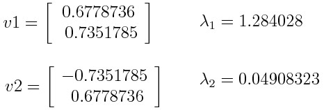
The eigenvectors and eigenvalues of this covariance matrix are:

Eigenvalue ( lambda_1 = 3.732 ), Eigenvector ( v_1 = begin{bmatrix} 0.615 0.789 end{bmatrix} )
Eigenvalue ( lambda_2 = 1.268 ), Eigenvector ( v_2 = begin{bmatrix} -0.789 0.615 end{bmatrix} )

Since ( lambda_1 > lambda_2 ), the first principal component (PC1) is ( v_1 ) and the second principal component (PC2) is ( v_2 ).

Principal Component Analysis Example

5.4. Step 4: Feature Vector Creation

Creating a feature vector involves selecting the principal components to keep based on their eigenvalues. This step is crucial for dimensionality reduction, as it determines which components will be used to represent the data.

5.4.1. Selecting Principal Components

Based on Eigenvalues: Principal components are selected based on their eigenvalues. Components with larger eigenvalues explain more variance in the data and are therefore more important.
Dimensionality Reduction: The goal is to reduce the number of dimensions while retaining as much variance as possible. This is achieved by discarding components with low eigenvalues.

5.4.2. Forming the Feature Vector

Matrix of Eigenvectors: The feature vector is a matrix that contains the eigenvectors of the selected principal components as columns.
Reduced Dimensionality: If you choose to keep only ( p ) eigenvectors out of ( n ), the final dataset will have only ( p ) dimensions.

5.4.3. Example of Feature Vector Creation

Continuing with the previous example, we have two eigenvectors:

( v_1 = begin{bmatrix} 0.615 0.789 end{bmatrix} ) with eigenvalue ( lambda_1 = 3.732 )
( v_2 = begin{bmatrix} -0.789 0.615 end{bmatrix} ) with eigenvalue ( lambda_2 = 1.268 )

If we decide to keep only the first principal component (PC1), the feature vector would be:

[
text{Feature Vector} = begin{bmatrix} 0.615 0.789 end{bmatrix}
]
This reduces the dimensionality of the data from 2 to 1.

5.4.4. Variance Explained

To determine how many components to keep, you can calculate the percentage of variance explained by each component:
[
text{Variance Explained} = frac{lambdai}{sum{j=1}^{n} lambda_j}
]
For our example:

Variance Explained by PC1 = ( frac{3.732}{3.732 + 1.268} = 0.7464 ) or 74.64%
Variance Explained by PC2 = ( frac{1.268}{3.732 + 1.268} = 0.2536 ) or 25.36%

This means that the first principal component explains 74.64% of the variance in the data.

5.5. Step 5: Data Transformation

In the final step, the data is transformed by recasting it along the axes of the principal components. This involves multiplying the original data by the feature vector to obtain the new data representation in the reduced dimensional space.

5.5.1. Transforming the Data

Reorienting the Data: The goal is to reorient the data from the original axes to the axes represented by the principal components.
Using the Feature Vector: The feature vector, which contains the eigenvectors of the selected principal components, is used to transform the data.

5.5.2. Mathematical Transformation

The transformed data ( text{Data}{text{transformed}} ) is obtained by multiplying the transpose of the original data ( text{Data}{text{original}}^T ) by the transpose of the feature vector ( text{Feature Vector}^T ):
[
text{Data}{text{transformed}} = text{Data}{text{original}}^T times text{Feature Vector}
]

5.5.3. Example of Data Transformation

Suppose we have the original data point ( x = begin{bmatrix} 2 3 end{bmatrix} ) and the feature vector ( text{Feature Vector} = begin{bmatrix} 0.615 0.789 end{bmatrix} ).

The transformed data point is:
[
text{Data}_{text{transformed}} = begin{bmatrix} 2 & 3 end{bmatrix} times begin{bmatrix} 0.615 0.789 end{bmatrix} = [2(0.615) + 3(0.789)] = [1.23 + 2.367] = [3.597]
]
So, the transformed data point is 3.597 in the reduced dimensional space.

An overview of principal component analysis (PCA).

6. What are the Benefits of Using PCA?

PCA offers several compelling benefits, making it a valuable tool in various domains, all of which are thoroughly explained and illustrated with examples at LEARNS.EDU.VN:

Reduced Complexity: Simplifies high-dimensional data, making it easier to analyze and interpret.
Improved Model Performance: Reduces overfitting and speeds up training in machine learning models.
Enhanced Visualization: Facilitates the creation of informative visualizations for data exploration.
Noise Reduction: Removes noise and irrelevant information from the data.
Feature Extraction: Extracts the most important features from the data, improving model accuracy.

7. What are the Limitations of PCA?

While PCA is a powerful technique, it has certain limitations that should be considered when applying it to real-world problems, limitations that LEARNS.EDU.VN addresses with alternative solutions and best practices:

Linearity Assumption: PCA assumes that the relationships between variables are linear, which may not be true for all datasets.
Sensitivity to Scaling: PCA is sensitive to the scaling of the original variables, requiring standardization as a preprocessing step.
Information Loss: Reducing the number of dimensions can result in some loss of information, particularly if the discarded components contain important variance.
Interpretability: The principal components may not be easily interpretable in terms of the original variables.
Data Distribution: PCA works best when the data is normally distributed.

8. How to Evaluate the Performance of PCA?

Evaluating the performance of PCA involves assessing how well the reduced-dimensional data retains the important information from the original data. Here are several methods to evaluate PCA performance, methods that are clearly demonstrated at LEARNS.EDU.VN:

Explained Variance Ratio:
- Definition: The explained variance ratio measures the proportion of the dataset’s variance that each principal component captures.
- Calculation: For each principal component ( i ), the explained variance ratio ( text{EVR}_i ) is calculated as:
  [
  text{EVR}_i = frac{lambdai}{sum{j=1}^{n} lambda_j}
  ]
  where ( lambda_i ) is the eigenvalue of the ( i )-th principal component, and ( n ) is the total number of components.
- Interpretation: A high explained variance ratio indicates that the component captures a significant amount of information. Cumulative explained variance can be calculated by summing the explained variance ratios for the first ( k ) components, indicating the total variance retained by those components.
Reconstruction Error:
- Definition: Reconstruction error measures the difference between the original data and the data reconstructed from the reduced-dimensional representation.
- Calculation:
  1. Reduce Dimensions: Apply PCA to reduce the data to ( k ) principal components.
  2. Reconstruct Data: Reconstruct the original data from the reduced-dimensional representation.
  3. Calculate Error: Calculate the mean squared error (MSE) between the original and reconstructed data:
    [
    text{MSE} = frac{1}{n} sum_{i=1}^{n} |x_i – hat{x}_i|^2
    ]
    where ( x_i ) is the original data point, ( hat{x}_i ) is the reconstructed data point, and ( n ) is the number of data points.
- Interpretation: A low reconstruction error indicates that the reduced-dimensional representation preserves the important information in the data.
Visualization:
- Method: Visualize the data in the reduced-dimensional space (e.g., using a scatter plot for 2D or 3D).
- Interpretation: Check if the reduced-dimensional representation preserves the separation between different classes or clusters in the data. If the clusters are well-separated, PCA has effectively retained the important information.
Performance on Downstream Tasks:
- Method: Evaluate the performance of machine learning models trained on the reduced-dimensional data and compare it to the performance of models trained on the original data.
- Process:
  1. Split Data: Divide the dataset into training and testing sets.
  2. Apply PCA: Apply PCA to the training set to reduce the dimensions.
  3. Train Model: Train a machine learning model on the reduced-dimensional training data.
  4. Test Model: Evaluate the model on the reduced-dimensional testing data and the original testing data.
- Interpretation: If the model performs similarly on the reduced-dimensional data compared to the original data, PCA has effectively retained the important information for that task.
Scree Plot:
- Definition: A scree plot is a line plot of the eigenvalues in descending order. It helps to identify the “elbow point,” where the rate of decrease in eigenvalues slows down significantly.
- Interpretation: The components before the elbow point are typically retained, as they capture the most variance in the data.

9. Real-World Examples of PCA in Action

PCA is applied across various fields to simplify data, enhance analysis, and improve decision-making. Here are some real-world examples of how PCA is used in different domains, examples available for in-depth exploration at LEARNS.EDU.VN:

Image Compression:
- Application: PCA is used to reduce the size of image files while preserving essential image features.
- Process:
  1. Data Representation: Images are represented as matrices of pixel values.
  2. Apply PCA: PCA is applied to reduce the dimensionality of the pixel data, retaining the most important components.
  3. Reconstruction: The compressed image is reconstructed from the reduced-dimensional representation.
- Benefits: Reduced storage space, faster transmission times, and minimal loss of image quality.
Genomics and Bioinformatics:
- Application: PCA is used to analyze gene expression data and identify key genes that contribute to certain diseases or conditions.
- Process:
  1. Data Collection: Gene expression data is collected from microarray experiments or RNA sequencing.
  2. Apply PCA: PCA is applied to reduce the dimensionality of the gene expression data, highlighting the genes with the most significant variance.
  3. Identification: Key genes are identified based on their contribution to the principal components.
- Benefits: Identification of potential drug targets, improved understanding of disease mechanisms, and personalized medicine approaches.
Finance and Economics:
- Application: PCA is used to analyze financial data, such as stock prices and economic indicators, to identify key factors that drive market trends.
- Process:
  1. Data Collection: Financial data is collected from various sources, such as stock exchanges and economic databases.
  2. Apply PCA: PCA is applied to reduce the dimensionality of the financial data, identifying the most important factors.
  3. Analysis: Key factors, such as interest rates, inflation, and market sentiment, are analyzed to understand their impact on market trends.
- Benefits: Improved investment strategies, risk management, and economic forecasting.
Environmental Science:
- Application: PCA is used to analyze environmental data, such as air and water quality measurements, to identify pollution sources and assess environmental impact.
- Process:
  1. Data Collection: Environmental data is collected from various monitoring stations and sensors.
  2. Apply PCA: PCA is applied to reduce the dimensionality of the environmental data, identifying the most important pollutants and environmental factors.
  3. Source Identification: Pollution sources are identified based on their contribution to the principal components.
- Benefits: Effective pollution control measures, environmental monitoring, and sustainable resource management.
Sensor Data Analysis:
- Application: PCA is used to analyze data from sensors in various applications, such as IoT devices, wearable technology, and industrial equipment.
- Process:
  1. Data Collection: Sensor data is collected from various devices and systems.
  2. Apply PCA: PCA is applied to reduce the dimensionality of the sensor data, extracting the most important features and patterns.
  3. Anomaly Detection: Anomalies and abnormal patterns are detected based on deviations from the principal components.
- Benefits: Improved device performance, predictive maintenance, and enhanced system reliability.

10. Frequently Asked Questions (FAQs) about PCA

Here are some frequently asked questions about Principal Component Analysis (PCA), answered to provide a deeper understanding of this technique, with additional resources available at LEARNS.EDU.VN:

10.1. What does a PCA plot tell you?

A PCA plot shows the relationships between samples in a dataset in terms of the principal components. Each point represents a sample, and its position is determined by its scores on the first few principal components. The plot can reveal clusters, trends, and outliers in the data.

10.2. Why is PCA used in machine learning?

PCA is used to reduce the dimensionality of data, remove multicollinearity, and improve model performance. By reducing the number of features, PCA helps to prevent overfitting, speed up training, and enhance the interpretability of machine learning models.

10.3. How many principal components should I choose?

The number of principal components to choose depends on the amount of variance you want to retain and the specific application. You can use the explained variance ratio, scree plot, or performance on downstream tasks to determine the optimal number of components.

10.4. Is PCA a supervised or unsupervised learning technique?

PCA is an unsupervised learning technique because it does not require labeled data. It analyzes the structure of the data to identify the principal components without any prior knowledge of the class labels.

10.5. Can PCA be used for non-linear data?

PCA is a linear technique and may not be effective for non-linear data. In such cases, non-linear dimensionality reduction techniques, such as t-SNE or UMAP, may be more appropriate.

10.6. What is the difference between PCA and factor analysis?

PCA and factor analysis are both dimensionality reduction techniques, but they have different goals and assumptions. PCA aims to explain the variance in the data, while factor analysis aims to identify underlying factors that explain the correlations between variables.

10.7. How does PCA handle missing data?

PCA cannot handle missing data directly. You need to impute or remove the missing values before applying PCA.

10.8. Can PCA be used for feature selection?

Yes, PCA can be used for feature selection by selecting the original variables that contribute the most to the principal components.

10.9. What are the assumptions of PCA?

The main assumptions of PCA are linearity, normality, and equal variance. PCA works best when the relationships between variables are linear, the data is normally distributed, and the variables have equal variance.

10.10. How do I interpret the principal components?

Interpreting the principal components involves examining the eigenvectors and determining which original variables contribute the most to each component. You can also use domain knowledge to understand the meaning of the components in the context of your data.

Principal Component Analysis (PCA) is a powerful technique for dimensionality reduction and feature extraction, offering numerous benefits for data analysis and machine learning. By understanding the key steps, applications, and limitations of PCA, you can effectively leverage this technique to simplify complex datasets, improve model performance, and gain valuable insights, and you can learn more at LEARNS.EDU.VN!

Ready to take your machine learning skills to the next level? Visit LEARNS.EDU.VN today to explore our comprehensive resources and courses on PCA and other essential techniques. Unlock your potential and become a data analysis expert with our expert guidance and practical examples.

Address: 123 Education Way, Learnville, CA 90210, United States
WhatsApp: +1 555-555-1212
Website: learns.edu.vn

Visit us now and start your journey towards mastering machine learning!