Machine Learning Basics: Your Comprehensive Guide to Fundamental Concepts

Machine learning (ML) is a transformative branch of artificial intelligence (AI) that empowers computers to learn from data without explicit programming. By analyzing past experiences and identifying patterns within datasets, machine learning algorithms can make predictions, automate decisions, and improve their performance over time. This field is broadly categorized into supervised learning, unsupervised learning, and reinforcement learning, each offering unique approaches to problem-solving.

This article serves as an essential introduction to the fundamentals of machine learning. We will break down complex ideas into easily digestible concepts and explore the core techniques that form the bedrock of this exciting domain. Whether you’re a student, a budding data scientist, or simply curious about the technology shaping our future, this guide will equip you with a solid understanding of Machine Learning Basics.

Machine Learning Explained

At its core, machine learning is about enabling systems to learn from data. Instead of being explicitly instructed on how to perform a task, machine learning algorithms are trained on datasets, allowing them to identify patterns, extract insights, and make data-driven predictions or decisions. This capability to learn and adapt makes machine learning a powerful tool across diverse industries.

Arthur Samuel, a pioneer in artificial intelligence, famously defined machine learning in 1959 as giving “computers the ability to learn without being explicitly programmed.” This definition highlights the key aspect of ML: learning from data rather than relying on hard-coded rules.

Building on this, Tom M. Mitchell provided a more technical definition in his 1997 paper: “A computer program is said to learn from experience E with respect to some class of tasks T and performance measure P, if its performance at tasks in T, as measured by P, improves with experience E.”

Let’s illustrate this with an example: handwriting recognition.

• Task (T): Identifying and classifying handwritten words from images.
• Performance Measure (P): Accuracy, measured by the percentage of correctly classified words.
• Training Experience (E): A dataset containing images of handwritten words paired with their correct classifications.

The machine learning system learns from the training dataset (E) to improve its performance (P) on the task of handwriting recognition (T). A dataset is simply a collection of examples, where each example is described by a set of features.

Common Types of Machine Learning

Machine learning is commonly divided into three primary types, each suited for different types of problems and data: Supervised learning, unsupervised learning, and reinforcement learning.

1. Supervised Learning

Supervised learning is characterized by the use of labeled datasets. In this approach, the machine learning algorithm is trained on examples where each input is paired with a corresponding output label or target. This “supervision” allows the algorithm to learn the relationship between inputs and outputs and generalize this knowledge to new, unseen data.

Two fundamental tasks in supervised learning are classification and regression.

Classification: In classification tasks, the goal is to predict the category or class to which a new data point belongs. The model learns to assign discrete labels based on the input features. Examples of classification include:

• Spam Email Detection: Classifying emails as “spam” or “not spam.”
• Image Recognition: Identifying objects in images, such as “cat,” “dog,” or “car.”
• Medical Diagnosis: Predicting whether a patient has a certain disease based on medical test results.

Regression: Regression tasks involve predicting a continuous numerical value. The model learns to map input features to a continuous output variable. Examples of regression include:

• Predicting House Prices: Estimating the price of a house based on features like size, location, and number of bedrooms.
• Sales Forecasting: Predicting future sales based on historical sales data and marketing spend.
• Stock Price Prediction: Forecasting stock prices based on market trends and company performance.

2. Unsupervised Learning

Unsupervised learning deals with unlabeled data. The algorithm is tasked with finding patterns, structures, and relationships within the data without explicit guidance. The system attempts to understand the inherent organization of the data itself.

Clustering is a prominent unsupervised learning technique.

Clustering: Clustering algorithms group similar data points together based on their features. The algorithm identifies natural clusters or groupings within the data. Examples of clustering include:

• Customer Segmentation: Grouping customers based on their purchasing behavior to personalize marketing efforts.
• Document Categorization: Organizing news articles or documents into thematic groups.
• Anomaly Detection: Identifying unusual patterns or outliers in datasets, such as fraudulent transactions.

3. Reinforcement Learning

Reinforcement learning is distinct from supervised and unsupervised learning. It involves training an agent to interact with an environment to achieve a specific goal. The agent learns through trial and error, receiving rewards or penalties based on its actions. The objective is to maximize cumulative rewards over time.

Reinforcement learning is inspired by behavioral psychology and is particularly well-suited for tasks where sequential decision-making is crucial. Examples include:

• Game Playing: Training AI agents to play games like chess, Go, or video games.
• Robotics: Developing robots that can learn to navigate environments, manipulate objects, or perform complex tasks.
• Resource Management: Optimizing resource allocation, such as managing power grids or traffic flow.

Visual representation of machine learning basics, highlighting different categories and applications.

Supervised Machine Learning Techniques: Regression

Regression techniques are fundamental to supervised learning, focusing on predicting continuous numerical values. They establish relationships between dependent variables (the values we want to predict) and independent variables (predictor variables).

Linear Regression and Logistic Regression are two of the most widely used regression techniques. Let’s delve into linear regression, along with essential concepts like gradient descent, overfitting, underfitting, regularization, hyperparameters, and cross-validation.

Linear Regression: Predicting Continuous Values

In linear regression, the goal is to model the relationship between variables using a linear equation. We aim to predict a dependent variable, y, based on one or more independent variables, represented as a vector X. The model assumes a linear relationship:

ŷ = WX + b

Where:

• ŷ is the predicted value.
• X is the vector of input features.
• W is the vector of weights or parameters, representing the influence of each feature on the prediction.
• b is the bias term, an intercept that shifts the line up or down.

The task (T) in linear regression is to accurately predict y from X. To assess the model’s performance (P), we need to measure the error between the predicted values and the actual values.

Measuring Model Performance: Error Calculation

For each data point i, the error is calculated as the difference between the actual value (y) and the predicted value (ŷ):

Error calculation for each example i.

To quantify the overall error of the model, we use loss functions. Two common loss functions for linear regression are Mean Absolute Error (MAE) and Mean Squared Error (MSE).

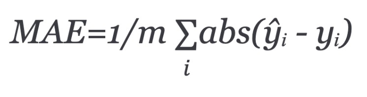
Mean Absolute Error (MAE)

MAE calculates the average of the absolute differences between predictions and actual values.

Mean Squared Error (MSE)

MSE calculates the average of the squared differences between predictions and actual values. Squaring the errors penalizes larger errors more heavily.

Mean squared error equation.

The factor of 1/2 in the MSE formula is for mathematical convenience in gradient descent calculations, as it simplifies the derivative.

Gradient Descent: Optimizing Model Parameters

The primary objective in training a machine learning model is to find the optimal values for the weights (W) and bias (b) that minimize the chosen loss function (MAE or MSE). Gradient descent is a widely used optimization algorithm to achieve this.

Gradient descent is an iterative process. It starts with random initial values for the model parameters and then iteratively adjusts them to reduce the loss. It works by calculating the gradient of the loss function with respect to the parameters. The gradient indicates the direction of the steepest ascent of the loss function. To minimize the loss, we move in the opposite direction of the gradient.

Gradient Descent Algorithm Steps:

1. Initialization: Initialize weights (W) and bias (b) randomly.
2. Iteration: Repeat until convergence (minimum loss):
   • Calculate the gradient of the loss function J(W) with respect to each parameter Wj.
   • Update each parameter Wj in the opposite direction of the gradient:

Minimum cost equation.

Where:
* *α* (alpha) is the learning rate, a hyperparameter that controls the step size in each iteration. A larger learning rate can lead to faster convergence but may overshoot the minimum. A smaller learning rate ensures more stable convergence but can be slower.

Types of Gradient Descent:

There are three main variations of gradient descent, differing in how much data is used to calculate the gradient in each iteration:

1. Batch Gradient Descent: Uses the entire training dataset to calculate the gradient in each iteration. This method is computationally expensive for large datasets but provides a stable gradient estimate.
2. Mini-Batch Gradient Descent: Divides the training data into smaller batches (mini-batches) and calculates the gradient using each mini-batch in each iteration. This is a compromise between batch and stochastic gradient descent, offering a balance of computational efficiency and gradient stability.
3. Stochastic Gradient Descent (SGD): Uses only a single randomly selected training example to calculate the gradient in each iteration. SGD is computationally very efficient and can converge faster than batch gradient descent, especially for large datasets. However, the gradient estimate is noisy, and convergence can be less stable.

Logistic Regression: Predicting Probabilities for Classification

Logistic regression, despite its name, is a classification algorithm. It’s used when the dependent variable is categorical, representing probabilities of belonging to different classes. Unlike linear regression, which predicts continuous values, logistic regression predicts the probability of a binary outcome (e.g., 0 or 1, yes or no).

In logistic regression, the output is constrained to be between 0 and 1, representing probabilities. This is achieved by using the sigmoid function (also known as the logistic function) to transform the linear combination of inputs.

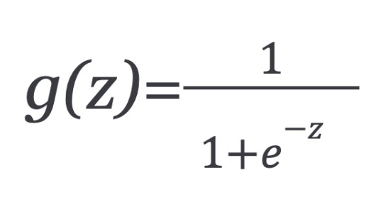
Sigmoid Function:

Sigmoid function equation.

The sigmoid function, g(z), takes any real number z and maps it to a value between 0 and 1. This makes it ideal for modeling probabilities.

In logistic regression, we model the probability of the positive class (e.g., class 1) as:

Logistic function.

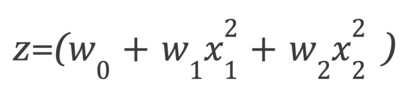
Where z is a linear combination of input features:

Z equation for linear function.

g(x) is interpreted as the probability that the output belongs to the positive class (class 1). For example, if g(x) = 0.7, it means there is a 70% probability that the output is class 1, and therefore a 30% probability that it is class 0 (the complement).

Cost Function for Logistic Regression

We cannot use the same MSE cost function as in linear regression for logistic regression. The sigmoid function introduces non-convexity, leading to multiple local minima and hindering gradient descent’s ability to find the global minimum.

To ensure a convex cost function for logistic regression, we use a cost function based on the logarithm of the sigmoid function, known as the cross-entropy loss or log loss.

Cost function for linear regression.

This cost function can be written in a more compact form:

cost function rewritten

Finally, the cost function for logistic regression is:

Cost function for logistic regression.

This cost function is convex, guaranteeing that gradient descent will converge to the global minimum, finding the optimal model parameters.

Understanding Underfitting and Overfitting in Machine Learning

When building machine learning models, we aim for a model that generalizes well to unseen data. However, models can sometimes either be too simple (underfitting) or too complex (overfitting), hindering their generalization ability.

Underfitting:

Underfitting occurs when a model is too simple to capture the underlying patterns in the data. It fails to learn the training data adequately and, consequently, performs poorly on both the training data and unseen data. An underfit model has high bias.

Characteristics of Underfitting:

• High training error: The model performs poorly on the training data.
• High validation/test error: The model also performs poorly on unseen data.
• Simple model: The model is not complex enough to capture the data’s complexity.

Overfitting:

Overfitting occurs when a model is too complex and learns the training data too well, including noise and random fluctuations. While it performs exceptionally well on the training data, it fails to generalize to unseen data. An overfit model has high variance.

Characteristics of Overfitting:

• Low training error: The model performs very well on the training data.
• High validation/test error: The model performs poorly on unseen data.
• Complex model: The model is too complex and has learned noise in the training data.

Addressing Overfitting:

Several techniques can mitigate overfitting:

1. Reduce the Number of Features: Feature selection involves choosing the most relevant features and discarding less important ones. This simplifies the model and reduces its complexity. However, it’s crucial to avoid discarding features that might contain valuable information.
2. Regularization: Regularization techniques add a penalty term to the loss function, discouraging the model from learning overly complex relationships. This constrains the model’s parameters and reduces overfitting.
3. Early Stopping: During iterative training algorithms like gradient descent, early stopping monitors the model’s performance on a validation set. Training is stopped when the validation performance starts to degrade, preventing the model from overfitting.
4. Increase Training Data: Providing more training data can help the model learn more robust patterns and reduce overfitting.

Regularization in Machine Learning: Controlling Model Complexity

Regularization is a crucial technique to prevent overfitting by adding a penalty to the loss function. This penalty discourages the model from assigning excessively large weights to features, effectively simplifying the model and improving its generalization ability.

Regularization can be applied to both linear and logistic regression.

Linear Regression with Regularization

In linear regression with regularization, we modify the error function by adding a regularization term. A common form of regularization is L2 regularization (Ridge Regression), which adds the sum of squared weights to the error function:

Linear regression error function.

Where:

• λ (lambda) is the regularization parameter, controlling the strength of the regularization. A larger λ imposes a stronger penalty on large weights, leading to more regularization.

To minimize this regularized error function, we use gradient descent with a modified update rule:

Repeat gradient descent algorithm to convergence.

Expanding the equation:

Equation continued to convergence.

This can be rewritten as:

Manipulation of above equation.

Notice that the first term, (1 – αλ/m), is always less than 1. This term effectively shrinks the weight Wj in each iteration.

First term is always less than 1 equation.

L2 regularization effectively reduces the magnitude of the weights, preventing them from becoming too large and thus reducing overfitting.

Logistic Regression with Regularization

Similarly, we can apply regularization to logistic regression by adding a penalty term to its cost function:

Cost function of logistic regression with regularization.

The gradient descent update rule for logistic regression with regularization is:

Equation continued until convergence with regularization.

Expanding further:

Equation continued with regularization.

L1 and L2 Regularization: Ridge vs. Lasso

The regularization term we’ve discussed so far is L2 regularization, also known as Ridge Regression. It penalizes the squared magnitude of the weights.

L2 Regularization (Ridge Regression):

L2 equation

Another common regularization technique is L1 regularization, also known as Lasso Regression. L1 regularization penalizes the absolute value of the weights.

L1 Regularization (Lasso Regression):

L1 equation.

Key Differences Between L1 and L2 Regularization:

Feature	L1 Regularization (Lasso)	L2 Regularization (Ridge)
Penalty	Absolute value of weights	Squared value of weights
Weight Shrinkage	Shrinks some weights to zero	Shrinks all weights
Feature Selection	Performs feature selection	No feature selection
Sparsity	Induces sparsity	Does not induce sparsity

• L2 Regularization: Shrinks all weights proportionally but rarely forces weights to be exactly zero. It reduces the impact of less important features but keeps them in the model.
• L1 Regularization: Can shrink some weights to exactly zero, effectively performing feature selection. This can lead to simpler and more interpretable models, especially when dealing with high-dimensional data with many irrelevant features.

Hyperparameters: Tuning Model Behavior

Hyperparameters are parameters that are set before the training process begins. They control the learning process and the model’s structure. Unlike model parameters (weights and biases), which are learned from the data, hyperparameters are set externally.

Examples of hyperparameters we’ve encountered include:

• Learning Rate (α): In gradient descent, controls the step size during optimization.
• Regularization Parameter (λ): In regularization, controls the strength of the penalty.

Choosing appropriate hyperparameter values is crucial for achieving optimal model performance.

Cross-Validation: Evaluating and Selecting Models

Cross-validation is a powerful technique for evaluating model performance and selecting the best hyperparameters. It helps to prevent overfitting during model selection and provides a more reliable estimate of a model’s generalization ability.

The Need for Cross-Validation:

If we repeatedly use the same test dataset to evaluate different models and hyperparameter settings, the test set effectively becomes part of the training process, leading to overfitting to the test set. Cross-validation addresses this by using separate validation sets for model selection.

Data Splitting for Cross-Validation:

To perform cross-validation, we typically divide the dataset into three sets:

1. Training Set: Used to train the machine learning models.
2. Validation Set: Used to evaluate different models and hyperparameter settings during model selection.
3. Test Set: Held-out dataset used for final evaluation of the chosen model after model selection.

K-Fold Cross-Validation:

K-fold cross-validation is a widely used technique when the amount of data is limited. It maximizes the use of available data for both training and validation.

7 Steps of K-Fold Cross-Validation (for Hyperparameter Selection):

1. Split Data: Divide the training data into K equal-sized folds (e.g., K=5 or K=10).
2. Hyperparameter Grid: Define a set of hyperparameter values to evaluate.
3. Iterate through Hyperparameters: For each set of hyperparameters:
   4. Inner Loop (K-Fold Validation):
   • For each fold k from 1 to K:
     • Train the model on the remaining K-1 folds.
     • Evaluate the model’s performance on the k-th fold (validation fold).
   • Calculate the average performance metric across all K folds. This is the cross-validation performance for the current hyperparameter set.
4. Select Best Hyperparameters: Choose the hyperparameter set that yields the best average cross-validation performance.
5. Train Final Model: Train the final model using the selected hyperparameters on the entire training dataset.
6. Evaluate on Test Set: Evaluate the final model’s performance on the held-out test set to get an unbiased estimate of its generalization ability.

Cross-validation allows us to tune hyperparameters and select models using only the training data, preserving the test set for a truly independent final evaluation.

Understanding Feature Importance in Machine Learning – Further explore related concepts in machine learning.

Frequently Asked Questions

What is the difference between AI and ML?

Artificial intelligence (AI) is the broader field encompassing the creation of intelligent machines capable of mimicking human cognitive abilities like learning, problem-solving, and decision-making. Machine learning (ML) is a specific approach within AI that focuses on enabling machines to learn from data and improve their performance on tasks without explicit programming for every step. ML is a tool used to achieve AI.

What are the 4 types of machine learning?

While often categorized into three, machine learning is sometimes described as having four types:

1. Supervised Learning: Learning from labeled data.
2. Unsupervised Learning: Learning from unlabeled data.
3. Semi-Supervised Learning: Learning from a combination of labeled and unlabeled data.
4. Reinforcement Learning: Learning through interaction with an environment and reward feedback.

What’s the difference between machine learning and deep learning?

Machine learning is a broad field encompassing various algorithms that enable machines to learn from data. Traditional machine learning often requires feature engineering and human intervention to guide the learning process. Deep learning is a subfield of machine learning that utilizes artificial neural networks with multiple layers (deep neural networks). Deep learning excels at automatically learning complex features from raw data, often requiring less human intervention compared to traditional machine learning for feature engineering and model refinement. Deep learning is particularly powerful for complex tasks like image recognition and natural language processing.