Machine Learning Decision Tree: A Comprehensive Guide for Beginners

Decision trees are fundamental models in machine learning, renowned for their interpretability and versatility. In our previous exploration of decision trees, we laid the groundwork by understanding how they visually represent decision-making processes. We learned that these tree-like structures use internal nodes for feature-based tests, branches for decision rules, and leaf nodes to deliver predictions. This foundational knowledge is essential, and now, we’re advancing to a deeper dive into the practical implementation of decision trees within machine learning.

Let’s elevate our understanding and explore the mechanics of training a decision tree model, making accurate predictions, and effectively evaluating its performance in real-world scenarios.

Understanding the Decision Tree Structure in Machine Learning

A decision tree stands out as a powerful supervised learning algorithm, adept at tackling both classification and regression challenges. It elegantly models decisions using a tree-like structure, where each component plays a crucial role:

Internal Nodes: These represent attribute tests. They pose questions about the features of the data.
Branches: These symbolize attribute values or outcomes of the tests, guiding the path down the tree.
Leaf Nodes: These are the endpoints, representing the final decisions or predictions based on the traversed path.

Decision trees are highly valued in the machine learning community for their adaptability, clear interpretability, and broad applicability in predictive modeling. They offer a transparent approach to understanding the decision-making process behind predictions.

Before moving forward, grasping the intuition behind decision trees is crucial for a deeper understanding of their application and effectiveness.

The Intuition Behind Decision Trees

To simplify the concept, let’s consider a relatable example: deciding whether to go for a bike ride.

Step 1 – Root Node: Initial Question: “Is it a sunny day?” If the answer is yes, it’s more likely you’ll consider a bike ride. If no, you’ll proceed to the next question.
Step 2 – Internal Nodes: Further Questions: If it’s not sunny, you might ask: “Is it a weekend?” Weekends often mean more leisure time for activities. If yes, you might still consider a bike ride; if no, perhaps not.
Step 3 – Leaf Node: Final Decision: Based on your answers, you decide whether to go for a bike ride or choose another activity.

This simple scenario illustrates the core intuition of a decision tree: breaking down complex decisions into a series of simpler, sequential questions.

The Step-by-Step Approach in Decision Trees

Decision trees utilize a tree representation to solve problems. In this structure, each leaf node corresponds to a class label, indicating the predicted outcome, while the internal nodes of the tree represent the attributes or features that lead to these outcomes. Decision trees are capable of representing any boolean function on discrete attributes, making them a versatile tool.

Example: Predicting if Someone Enjoys Action Movies

Let’s predict whether a person enjoys action movies based on their age and gender. Here’s how a decision tree would approach this:

Start with the Root Question (Age):
- The initial question: “Is the person’s age less than 25?”
- Yes: Proceed to the left branch.
- No: Proceed to the right branch.
Branch Based on Age:
- If the person is younger than 25, they are likely to enjoy action movies (e.g., +1 prediction score).
- If the person is 25 or older, ask the next question: “Is the person male?”
Branch Based on Gender (For Age 25+):
- If the person is male, they might enjoy action movies (e.g., +0.5 prediction score).
- If the person is not male, they are less likely to enjoy action movies (e.g., -0.2 prediction score).

This example simplifies how a decision tree uses a series of questions to arrive at a prediction. In more complex scenarios, multiple decision trees can be combined for more robust predictions.

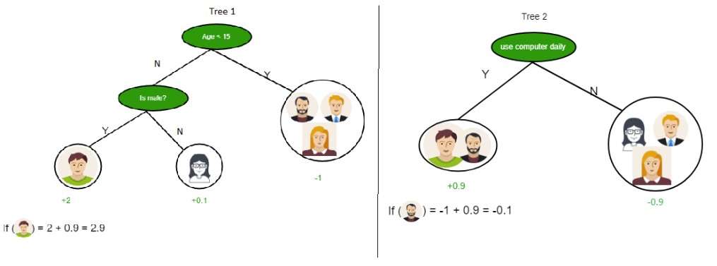
Combining Multiple Decision Trees for Enhanced Prediction

Consider using two decision trees to predict movie preferences for a more nuanced approach.

Tree 1: Age and Gender

This tree starts by evaluating age and then gender:
- “Is the person’s age less than 25?”
  - Yes: Assign a score of +1.
  - No: Proceed to the next question.
- “Is the person male?”
  - Yes: Add a score of +0.5.
  - No: Subtract a score of -0.2.

Tree 2: Genre Preference

The second tree focuses on preferred movie genres:
- “Does the person prefer action or comedy movies?”
  - Action: Assign a score of +0.8.
  - Comedy: Assign a score of -0.5.

Final Prediction

The combined prediction score is the sum of scores from both trees. This ensemble approach often yields more accurate and reliable predictions compared to a single decision tree.

Attribute Selection Measures: Information Gain and Gini Index

Now that we’ve explored the basic intuition and approach of decision trees, let’s delve into the crucial attribute selection measures that guide tree construction.

Two primary attribute selection measures are widely used in decision trees:

Information Gain
Gini Index

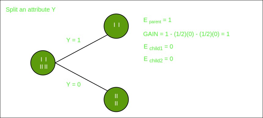
1. Information Gain

Information Gain is a measure that quantifies the effectiveness of an attribute in classifying data. It reflects the reduction in entropy (or uncertainty) achieved by partitioning the data based on a given attribute. A higher Information Gain indicates a more effective attribute for splitting data.

For instance, if splitting a group of moviegoers by “age group” perfectly separates those who prefer action movies from those who don’t, the Information Gain would be high. This attribute (age group) is then highly informative for making predictions.

Mathematically, Information Gain is calculated as:

Gain(S, A) = Entropy(S) - sum_{v in Values(A)}frac{|S_{v}|}{|S|} cdot Entropy(S_{v})

Where:

S is the set of data instances.
A is the attribute.
Values(A) is the set of all possible values of attribute A.
S_v is the subset of S for which attribute A has value v.
|S| and |S_v| are the number of instances in S and S_v respectively.
Entropy(S) is the entropy of dataset S.

Entropy, in this context, measures the impurity or disorder of a dataset. High entropy signifies a dataset with mixed classes, while low entropy indicates a dataset dominated by a single class.

For example, in a movie preference dataset, if you have an equal number of action movie enthusiasts and non-enthusiasts, the entropy is high, reflecting uncertainty. If, however, almost everyone prefers action movies, the entropy is low, indicating high certainty.

The formula for Entropy H(X) is:

H(X) = - sum_{i=1}^{n} p_i log_2(p_i)

Where p_i is the proportion of data points belonging to class i.

Example Calculation of Entropy:

Consider a dataset X = {action, action, action, comedy, comedy, comedy, comedy, comedy}.

Total instances: 8
Instances of ‘comedy’: 5
Instances of ‘action’: 3

The entropy H(X) is calculated as:

H(X) = - [ (3/8) log_2(3/8) + (5/8) log_2(5/8) ] ≈ 0.954

This entropy value indicates a moderate level of impurity in the dataset, as it contains a mix of both ‘action’ and ‘comedy’ preferences.

Building Decision Trees with Information Gain: Key Steps

Start at the Root: Begin with all training instances at the root node.
Attribute Selection: Use Information Gain to determine the best attribute for splitting the data at each node.
No Attribute Repetition: Ensure no attribute is repeated along any root-to-leaf path when dealing with discrete attributes.
Recursive Tree Building: Recursively construct each subtree for subsets of training instances, based on attribute values.
Leaf Node Labeling:
- If all instances in a subset belong to the same class, label the node as that class.
- If no attributes remain for splitting, label the node with the majority class of the instances at that node.
- If a subset is empty, label with the majority class from the parent node’s instances.

Example: Constructing a Decision Tree using Information Gain

Consider a training dataset for movie preference prediction:

Age Group	Gender	Genre Preference	Movie Preference
Young	Male	Action	Yes
Young	Female	Action	Yes
Senior	Female	Comedy	No
Senior	Male	Drama	No

Decision Tree Example for Movie Preference

To build a decision tree, we calculate the Information Gain for each attribute.

Split on ‘Age Group’

Split on ‘Gender’

Split on ‘Genre Preference’

From these calculations, suppose ‘Genre Preference’ yields the highest Information Gain. Thus, ‘Genre Preference’ becomes the root node. Splitting by ‘Genre Preference’ may directly lead to pure subsets (all ‘Yes’ or all ‘No’ for Movie Preference), eliminating the need for further splits.

The resulting simplified decision tree might look like this:

2. Gini Index

The Gini Index is another critical metric used in decision trees to evaluate the impurity of a dataset partition. It measures the probability of misclassifying a randomly chosen element if it were randomly labeled according to the class distribution in the subset. A lower Gini Index indicates higher purity, and attributes with lower Gini indices are preferred for splitting nodes.

Scikit-learn, a popular machine learning library, supports “gini” as a criterion for the Gini Index and uses it by default for decision tree classifiers.

For example, in movie preference prediction, if a group overwhelmingly prefers action movies (e.g., 90% “Yes”), the Gini Index is low, close to 0, signifying high purity. If the group is evenly split (50% “Yes” and 50% “No”), the Gini Index is higher, around 0.5, indicating greater impurity.

The formula for the Gini Index is:

Gini = 1 - sum_{i=1}^{n} p_i^2

Where p_i is the proportion of instances of class i in the dataset.

Key Features of the Gini Index:

Calculated by summing the squared probabilities of each class and subtracting from 1.
Lower Gini Index implies a more homogeneous distribution, while higher indicates heterogeneity.
Used to assess split quality by comparing parent node impurity to the weighted impurity of child nodes.
Computationally faster and more sensitive to changes in class probabilities compared to entropy.
May favor splits into equally sized child nodes, which may not always be optimal for accuracy.

The choice between Gini Index and Information Gain often depends on the specific dataset and problem, and empirical testing is usually recommended to determine the best measure.

Real-world Use Case: Step-by-Step Decision Tree Application

Let’s walk through a real-life scenario to understand how decision trees are applied practically. Imagine predicting customer churn for a streaming service.

Step 1: Start with the Entire Customer Dataset

Begin with all customer data, considering this the root node of our decision tree. This dataset includes features like viewing hours, subscription type, account age, and churn status (yes/no).

Step 2: Select the Best Attribute to Split (Root Node)

Choose the most informative attribute to split the dataset. For instance, “viewing hours per week” might be a strong predictor of churn. We would use Information Gain or Gini Index to evaluate each attribute and select the one that best separates churned from non-churned customers. Let’s say “viewing hours” is chosen as the root.

Step 3: Divide Data into Subsets Based on Attribute Values

Split the dataset based on the chosen attribute. For “viewing hours,” we might create branches like:

Less than 10 hours per week.
10-25 hours per week.
More than 25 hours per week.

Step 4: Recursive Splitting for Subsets if Necessary

For each subset, determine if further splitting is needed. If a subset still contains a mix of churned and non-churned customers, apply the attribute selection process again. For example, within the “less than 10 hours” subset, “subscription type” (basic/premium) could be the next attribute to split on.

For “less than 10 hours” & “basic subscription” – higher churn risk.
For “less than 10 hours” & “premium subscription” – lower churn risk.

Step 5: Assign Leaf Nodes (Churn Prediction)

When a subset becomes sufficiently pure (mostly churned or mostly non-churned customers), it becomes a leaf node, labeled with the predicted outcome (e.g., “Churn,” “No Churn”).

“More than 25 hours viewing” → “No Churn”.
“Less than 10 hours viewing” & “basic subscription” → “Churn”.

Step 6: Use the Decision Tree for Predictions

To predict churn for a new customer, traverse the tree based on their attributes. For example, if a new customer views 8 hours per week and has a basic subscription:

Start at the root (“viewing hours”).
Follow the “less than 10 hours” branch.
Then follow the “basic subscription” branch.
Result: Predict “Churn.”

This step-by-step process illustrates how decision trees break down complex prediction problems into manageable, interpretable steps, leading to a final decision.

Conclusion

Decision trees are a cornerstone of machine learning, providing a clear and intuitive approach to modeling and predicting outcomes. Their tree-like structure offers interpretability, versatility, and ease of visualization, making them invaluable for both classification and regression tasks. While decision trees offer numerous advantages, including simplicity and ease of understanding, they also present challenges like potential overfitting. A solid grasp of their terminology, construction process, and attribute selection methods is crucial for effectively applying decision trees in various real-world scenarios.

Frequently Asked Questions (FAQs)

1. What are the main challenges in decision tree learning?

The primary challenges include overfitting, where trees become too complex and fit noise in the training data, leading to poor generalization. They can also be sensitive to small variations in the training data. Techniques like pruning, setting constraints on tree depth, and ensemble methods like Random Forests help mitigate these issues.

2. How do decision trees aid in decision-making?

Decision trees simplify complex decision-making by breaking down choices into a series of sequential, attribute-based questions. They provide a transparent and interpretable path from initial data to final decision, making them excellent tools for understanding the logic behind predictions.

3. What is the significance of maximum depth in a decision tree?

Maximum depth is a crucial hyperparameter that limits the depth of the tree. It controls the complexity of the model and is essential for preventing overfitting. A shallower tree might underfit, while a deeper tree is more prone to overfitting.

4. Can you explain the fundamental concept of a decision tree?

At its core, a decision tree is a supervised learning algorithm that models decisions based on input features. It creates a tree-like structure where each internal node tests an attribute, each branch represents an outcome of the test, and each leaf node holds a class label or prediction.

5. What role does entropy play in decision trees?

Entropy in decision trees measures the impurity or randomness of a dataset. It’s used to calculate Information Gain, guiding the algorithm to make splits that maximally reduce uncertainty and effectively classify data. Lower entropy after a split indicates better information gain and a more effective attribute for decision-making.

6. What are the key Hyperparameters of decision trees?

Max Depth: Limits the maximum depth of the tree to control complexity.

Min Samples Split: Sets the minimum number of samples required to split an internal node, preventing splits on small subsets.

Min Samples Leaf: Defines the minimum number of samples required in a leaf node, ensuring leaf nodes are not too specific.

Criterion: Specifies the function to measure the quality of a split, such as ‘gini’ for Gini Index or ‘entropy’ for Information Gain.

Next Article KNN vs Decision Tree in Machine Learning

Abhishek Sharma 44

Improve

Article Tags : Machine Learning Decision Tree

Practice Tags : machine-learning