Top Machine Learning Algorithms in 2024: A Comprehensive Guide

Machine Learning (ML) algorithms are the unsung heroes powering a vast array of applications we use daily, from Netflix’s personalized movie recommendations to sophisticated fraud detection systems in financial institutions. These algorithms are the core intelligence behind systems that can analyze complex datasets, predict future trends, and automate intricate decision-making processes. In a landscape brimming with diverse algorithms, a solid understanding of their individual strengths and ideal applications is indispensable, especially for professionals in Data Science, Artificial Intelligence (AI), and Machine Learning.

This article delves into the top machine learning algorithms in 2024, offering a detailed exploration of fundamental concepts and their practical implementations across various industries. Whether you are just starting your journey in data science or are a seasoned expert, mastering these algorithms is crucial for thriving in the ever-evolving field of machine learning.

What are Machine Learning Algorithms?

A Machine Learning Algorithm is essentially a set of rules or a sequence of steps that enables a computer to learn from data. Unlike traditional programming where explicit instructions are given, ML algorithms identify patterns within data, allowing them to make predictions or decisions without direct programming for every situation. As these algorithms are exposed to more data, their performance improves, mimicking the human learning process through examples and experience. This capability empowers computers to evolve and become increasingly intelligent over time.

Top 15 Machine Learning Algorithms for 2024

Certain Machine Learning Algorithms have become particularly prominent due to their effectiveness in tackling complex, real-world data challenges. The following list presents 15 of the top algorithms, ranked based on their performance, versatility, and utility across diverse tasks and large datasets.

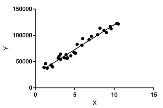
1. Linear Regression Algorithm

The Linear Regression Algorithm is a foundational supervised learning algorithm used to model the linear relationship between a dependent variable and one or more independent variables. It aims to find the best-fitting straight line (or hyperplane in higher dimensions) that describes how the dependent variable changes in response to changes in the independent variable(s). The independent variable is often referred to as the explanatory variable, while the dependent variable is the variable of interest that we want to predict or understand.

Consider using Linear Regression to predict house prices based on various features. Here’s how it would work:

Data Collection: Gather a comprehensive dataset of houses sold recently, including sale prices and relevant features such as square footage, number of bedrooms, number of bathrooms, and location.
Feature Selection: Identify the features that are likely to have a significant influence on house prices. These could include size, location, age, and amenities.
Model Training: Utilize the collected dataset to train the Linear Regression model. This involves finding the optimal coefficients for the linear equation that minimize the difference between the predicted prices and the actual sale prices in the dataset.
Price Prediction: Once trained, the model can be used to predict the price of a new house by inputting its features into the linear equation.
Model Evaluation: Assess the accuracy of the model using a separate dataset of houses (a test set) with known prices. Metrics like Mean Squared Error (MSE) or R-squared are used to evaluate the model’s performance.

By employing Linear Regression, real estate professionals and buyers can gain valuable insights into property valuation, making informed decisions in the housing market.

Time Complexity: [Tex]O(n times d^2)[/Tex]

Auxiliary Space: [Tex]O(d)[/Tex]

2. Logistic Regression Algorithm

While Linear Regression predicts continuous values, the Logistic Regression Algorithm is designed for binary classification tasks, dealing with discrete outcomes. It predicts the probability of a binary outcome (0 or 1, yes or no, true or false) based on a set of independent variables. Logistic regression is particularly useful when the dependent variable is categorical. The algorithm models the probability of an event occurring, classifying it as 1 if it occurs and 0 if it does not, based on the given predictor variables.

Let’s explore how Logistic Regression can predict customer churn for a subscription-based service:

Data Acquisition: Collect customer data including demographics (age, location), subscription details (plan type, sign-up date), usage patterns (frequency of use, features used), and payment history (payment failures, subscription duration).
Churn Factor Analysis: Analyze which factors are most indicative of churn. This could involve looking at engagement metrics, customer satisfaction scores (if available), and service usage patterns.
Model Training: Train the Logistic Regression model using the collected data. The model learns to associate certain customer characteristics and behaviors with the likelihood of churning.
Churn Probability Prediction: For new or existing customers, input their features into the trained model to calculate the probability of churn. Based on a chosen threshold (e.g., 0.5), customers are classified as either likely to churn (1) or not (0).
Performance Testing: Evaluate the model’s effectiveness on a separate dataset to assess its accuracy, precision, and recall. Adjustments to the model or threshold may be necessary to optimize performance.

By using Logistic Regression, businesses can proactively identify customers at risk of churn, enabling them to implement retention strategies and improve customer loyalty, similar to a proactive customer service manager identifying and addressing at-risk accounts.

Time Complexity: [Tex]O(n times d^2)[/Tex]

Auxiliary Space: [Tex] O(d)[/Tex]

3. Decision Trees Algorithm

The Decision Trees Algorithm is a versatile supervised machine learning algorithm applicable to both classification and regression problems. It constructs a tree-like model where each internal node represents a decision based on a feature, each branch represents the outcome of the decision, and each leaf node represents a class label (in classification) or a predicted value (in regression). Decision trees are intuitive and easy to interpret, making them a popular choice for understanding the decision-making process behind predictions.

Consider using a Decision Tree to predict whether a customer will purchase a product based on their characteristics:

Data Collection: Collect customer data, including attributes like age, income level, browsing history on the website, and past purchase behavior. Also, include a label indicating whether they made a purchase (yes/no).
Feature Importance Assessment: Determine which features are most influential in predicting purchases. Features like income and product interest are likely to be key predictors.
Tree Construction: Build a decision tree that recursively splits the dataset based on feature values. For example, the first split might be based on age, followed by income level for different age groups, and so on.
Purchase Prediction: Use the constructed decision tree to predict whether new customers will make a purchase by tracing their features down the tree to a leaf node, which will provide the purchase prediction (yes or no).
Accuracy Evaluation: Evaluate the model’s performance on a separate dataset to measure its accuracy. Adjustments to tree parameters (like depth or minimum samples per leaf) may be needed to optimize performance and prevent overfitting.

Decision Trees offer a clear and straightforward way to model decision processes, making them valuable for applications where interpretability is as important as prediction accuracy.

Time Complexity: [Tex]O(n times d times log(n))[/Tex]

Auxiliary Space: [Tex]O(n)[/Tex]

4. K-Nearest Neighbors Algorithm (KNN)

The K-Nearest Neighbors Algorithm (KNN) is a simple yet powerful non-parametric algorithm used for both classification and regression. It operates on the principle that similar data points are located close to each other. KNN classifies a new data point by considering the classes of its ‘K’ nearest neighbors in the feature space. The class with the majority among the K neighbors is assigned to the new data point. The choice of ‘K’ is crucial and can significantly impact the algorithm’s performance.

Let’s illustrate KNN with an example of classifying flowers into different species based on their features:

Flower Data Collection: Gather data on various flowers, including measurements of petal length, petal width, sepal length, sepal width, and the species label for each flower (e.g., Iris setosa, Iris versicolor, Iris virginica).
Feature Selection for Classification: Identify the most relevant features for distinguishing between flower species, such as petal and sepal dimensions.
Feature Scaling: Normalize the features to ensure that they all contribute equally to the distance calculations, as KNN is distance-based and sensitive to feature scales.
Classification of New Flowers: For a new, unclassified flower, calculate its distance to all flowers in the training dataset. Identify the ‘K’ nearest neighbors based on these distances. Classify the new flower based on the majority species among these neighbors.
Model Refinement: Test the model on a separate dataset to evaluate its classification accuracy. Experiment with different values of ‘K’ to find the optimal number of neighbors that yields the best performance.

Using KNN, one can effectively classify flowers, mirroring how a botanist might identify species by comparing characteristics to known samples.

Time Complexity: [Tex]O(n times d)[/Tex]

Auxiliary Space: [Tex]O(n times d)[/Tex]

5. Naive Bayes Classifier Algorithm

The Naive Bayes Classifier Algorithm is a probabilistic machine learning algorithm primarily used for classification tasks. It is based on Bayes’ theorem with the “naive” assumption of independence between features. Despite its simplicity and this assumption, Naive Bayes classifiers perform surprisingly well in many real-world applications, especially text classification and spam filtering due to its efficiency and effectiveness with high-dimensional data.

Consider how Gmail uses a Naive Bayes Classifier to categorize emails as “spam” or “not spam”:

Email Dataset Collection: Compile a labeled dataset of emails, categorized as either spam or legitimate (not spam).
Feature Extraction: Identify key features within emails that are indicative of spam. These features could include the presence of certain words (e.g., “free,” “discount,” “urgent”), the frequency of capital letters, the number of links, and sender information.
Classifier Training: Train a Naive Bayes Classifier using the email dataset. The algorithm calculates the probabilities of each feature appearing in spam and non-spam emails.
Spam Email Classification: For new incoming emails, analyze their features and compute the probability of them being spam or not spam based on the learned probabilities. Classify the email based on the higher probability.
Performance Tuning: Evaluate the classifier’s accuracy on a separate set of emails. Adjustments might involve refining the feature set or tweaking parameters to improve spam detection rates and reduce false positives.

Naive Bayes classifiers efficiently filter spam emails, saving users time and ensuring focus on important communications, much like a vigilant gatekeeper filtering out unwanted intrusions.

Time Complexity: T[Tex]O(nd)[/Tex]

Auxiliary Space: [Tex]O(c×d)[/Tex]

6. K-Means Clustering Algorithm

The K-Means Clustering Algorithm is a widely used unsupervised machine learning algorithm for partitioning data into distinct groups or clusters. It aims to minimize the within-cluster variance, meaning that data points within the same cluster are as similar as possible, while maximizing the variance between clusters. K-Means is effective for discovering underlying structures in data without labeled categories, making it invaluable in fields like market segmentation, image compression, and anomaly detection.

Let’s examine how K-Means Clustering can be used for customer segmentation in retail:

Customer Data Collection: Gather customer data, including demographics (age, gender, location), purchase history (items bought, purchase frequency, spending amounts), and website interaction data (pages visited, time spent browsing).
Determine Number of Segments: Decide on the number of customer segments to identify (e.g., high-value customers, occasional shoppers, budget-conscious buyers). This number, ‘K,’ is specified beforehand.
Centroid Initialization: Randomly select ‘K’ initial centroid points, each representing the center of a cluster.
Customer Assignment: Assign each customer to the nearest centroid based on a distance metric (e.g., Euclidean distance). This forms ‘K’ clusters.
Centroid Update: Recalculate the centroids of each cluster by averaging the data points within each cluster.
Iteration and Stabilization: Repeat steps 4 and 5 iteratively. In each iteration, customers are reassigned to clusters based on the new centroids, and centroids are updated based on the new cluster memberships. Continue until the centroids stabilize, meaning cluster assignments no longer change significantly.

Time Complexity: [Tex]O(n×k×i)[/Tex]

Auxiliary Space: [Tex]O(k×d)[/Tex]

7. Support Vector Machine Algorithm

The Support Vector Machine Algorithm (SVM) is a powerful supervised learning algorithm used for both classification and regression. It is particularly effective in high-dimensional spaces and is versatile due to the different kernel functions that can be used. In classification, SVM aims to find an optimal hyperplane that separates data points of different classes with the largest possible margin. Margin maximization is key to SVM’s robustness, as it tends to generalize well to unseen data.

Consider classifying images of cats and dogs using SVM:

Image Dataset Collection: Gather a dataset of images, labeled as either “cat” or “dog.”
Feature Extraction: Extract relevant features from each image that can distinguish between cats and dogs. These features could include color histograms, texture descriptors, and shape features.
SVM Training: Use the labeled dataset to train an SVM classifier. The training process involves finding the hyperplane that best separates cat images from dog images in the feature space, maximizing the margin between these classes.
Image Classification: For a new, unclassified image, extract the same features and use the trained SVM to classify it as either a cat or a dog based on which side of the hyperplane it falls.
Performance Assessment: Evaluate the SVM classifier on a separate test set of images to measure its accuracy in distinguishing between cats and dogs.

Time Complexity: Ranges from [Tex]O(n^2 times d) to O(n^3 times d)[/Tex]

Auxiliary Space: [Tex]O(n×d)[/Tex]

8. Apriori Algorithm

The Apriori Algorithm is a classic algorithm in data mining for association rule learning. It is used to identify frequent itemsets in transactional databases and then derive association rules. Association rules are IF-THEN statements that describe relationships between items. The Apriori algorithm is particularly useful in market basket analysis to understand which products are frequently purchased together, helping businesses make strategic decisions about product placement and marketing promotions.

Let’s see how the Apriori Algorithm is applied in market basket analysis in a grocery store:

Transaction Data Gathering: Collect transaction data from point-of-sale systems, listing all items purchased in each transaction.
Define Support and Confidence Thresholds: Set minimum support and confidence levels. Support is the frequency of an itemset, and confidence measures the reliability of a rule. These thresholds help filter out less significant itemsets and rules.
Frequent Itemset Mining: Use the Apriori algorithm to identify itemsets that meet the minimum support threshold. The algorithm iteratively finds frequent itemsets of increasing size, starting with single items and expanding to pairs, triplets, and so on.
Rule Generation: Generate association rules from the frequent itemsets. For example, a rule might be “IF {bread, butter} THEN {milk},” indicating that customers who buy bread and butter are also likely to buy milk.
Rule Analysis and Application: Analyze the generated rules for their usefulness and actionable insights. For instance, rules can inform product placement strategies (placing associated items near each other) or targeted marketing campaigns (offering discounts on associated items).

Time Complexity: [Tex]O(2^d)[/Tex].

Auxiliary Space: [Tex]O(2^d)[/Tex]

9. Random Forests Algorithm

The Random Forests Algorithm is an ensemble learning method based on decision trees. It addresses some limitations of single decision trees, such as overfitting and instability. Random Forests work by creating multiple decision trees during the training phase and outputting the mode of the classes (classification) or the mean prediction (regression) of the individual trees. This ensemble approach significantly improves accuracy and robustness compared to single decision trees. The algorithm leverages techniques like bagging (bootstrap aggregating) and feature randomness to ensure diversity among the trees.

Consider using a Random Forest to predict loan approval:

Loan Application Dataset: Collect a dataset of loan applications, including features like applicant income, credit score, loan amount requested, employment history, and past defaults. Include a label indicating whether the loan was approved or denied.
Data Preprocessing: Preprocess the data by handling missing values, encoding categorical variables (e.g., converting text categories into numerical form), and splitting the dataset into training and testing sets.
Forest Construction: Create a random forest by training multiple decision trees. Each tree is trained on a random subset of the data (bootstrapping) and using a random subset of features at each split (feature randomness).
Loan Approval Prediction: For a new loan application, each tree in the forest independently predicts whether the loan should be approved or denied. The Random Forest then aggregates these predictions (e.g., by majority vote for classification) to make a final prediction.
Model Performance Evaluation: Test the Random Forest model on a separate test set to evaluate its performance. Metrics like accuracy, precision, recall, and the area under the ROC curve (AUC) are used to assess the model’s effectiveness in predicting loan approvals.

Time Complexity: [Tex]O(t times n times d times log(n))[/Tex].

Auxiliary Space: [Tex]O(t times n)[/Tex]

10. Artificial Neural Networks Algorithm (ANN)

An Artificial Neural Network (ANN) is a computational model inspired by the structure and function of biological neural networks in the human brain. ANNs are composed of interconnected nodes called neurons, organized in layers. These networks can learn complex patterns from data and are used for a wide range of tasks, including classification, regression, pattern recognition, and more recently, in deep learning architectures for complex problems like image recognition and natural language processing.

Let’s illustrate ANN application with image recognition:

Image Dataset Preparation: Gather a large, labeled dataset of images. For example, for object recognition, the dataset might contain images of various objects like cars, trees, and animals, with each image labeled with the object it contains.
Data Preprocessing and Splitting: Preprocess the images, which might include resizing, normalization, and augmentation. Split the dataset into training, validation, and testing sets. The training set is used to train the network, the validation set to tune hyperparameters and monitor overfitting, and the test set to evaluate the final model performance.
Network Architecture Design: Design the architecture of the ANN. This involves deciding on the number of layers, the types of layers (e.g., convolutional layers, fully connected layers), the number of neurons in each layer, and the activation functions. For image recognition, Convolutional Neural Networks (CNNs) are often used.
Network Training: Train the ANN using the training dataset. This involves feeding the images through the network, calculating the output, comparing it to the true label, and adjusting the network’s weights using backpropagation and an optimization algorithm (like stochastic gradient descent) to minimize the loss function.
Performance Evaluation and Deployment: Evaluate the trained ANN on the validation and testing sets to measure its performance. Metrics like accuracy, precision, recall, and F1-score are used. Once satisfactory performance is achieved, the ANN can be deployed for real-world image recognition tasks.

Time Complexity: [Tex]O(e times n times l times d)[/Tex]

Auxiliary Space: [Tex]O(l times d^2)[/Tex]

11. Principal Component Analysis (PCA)

Principal Component Analysis (PCA) is a dimensionality reduction technique that transforms high-dimensional datasets into lower dimensions while retaining as much variance as possible. PCA identifies principal components, which are new uncorrelated variables that are linear combinations of the original variables, ordered by the amount of variance they explain. PCA is widely used for feature extraction, data visualization, and noise reduction, simplifying complex datasets and improving the performance of machine learning models.

Consider using PCA to reduce the dimensionality of a dataset for visualization:

Dataset Collection: Gather a dataset with a large number of features (dimensions). For example, a dataset of gene expression data, where each gene is a dimension.
Data Preprocessing: Normalize or standardize the data to ensure that each feature contributes equally to the analysis, preventing features with larger scales from dominating.
Covariance Matrix Calculation: Calculate the covariance matrix of the dataset to understand the relationships between different features.
Eigenvalue and Eigenvector Computation: Compute the eigenvalues and eigenvectors of the covariance matrix. Eigenvectors represent the principal components, and eigenvalues indicate the variance explained by each principal component.
Principal Component Selection: Select the top ‘k’ principal components corresponding to the largest eigenvalues. These components capture the most variance in the data and are used to reduce dimensionality.
Data Transformation: Project the original data onto the subspace spanned by the selected principal components. This yields a lower-dimensional representation of the data, which can be visualized in 2D or 3D, or used as input for other machine learning algorithms.

Time Complexity:[Tex]O(n⋅m^2+m^3)[/Tex]

Auxiliary Space:[Tex]O(m^2)[/Tex]

12. AdaBoost (Adaptive Boosting)

AdaBoost (Adaptive Boosting) is a boosting ensemble learning algorithm that combines multiple weak learners to create a strong classifier. It works iteratively, with each iteration focusing on correcting the misclassifications of the previous learners. AdaBoost assigns weights to each data point and adjusts these weights at each step, giving more weight to misclassified instances so that subsequent weak learners focus more on these difficult instances. This adaptive approach makes AdaBoost highly effective in improving the accuracy of weak classifiers.

Let’s see how AdaBoost can enhance the accuracy of a simple classifier for spam detection:

Labeled Email Dataset: Collect a dataset of emails, labeled as spam or not spam.
Initialize Weights: Assign equal weights to all emails in the training dataset.
Iterative Training of Weak Classifiers: Iteratively train weak classifiers (e.g., decision stumps, which are shallow decision trees) on the weighted dataset. In each iteration:
- Train a weak classifier that best classifies the weighted data.
- Calculate the error rate of the weak classifier.
- Calculate a weight for the weak classifier based on its error rate; more accurate classifiers get higher weights.
- Update the weights of the training instances. Increase the weights of misclassified instances so that the next weak classifier focuses more on them.
Combine Weak Classifiers: Combine the predictions of all weak classifiers into a final prediction. The combination is done by weighted voting, where each weak classifier’s vote is weighted by its calculated weight.
Performance Evaluation: Evaluate the AdaBoost classifier on a separate dataset to measure its accuracy, precision, and recall in spam detection.

Time Complexity: [Tex]O(M⋅n)[/Tex]

Auxiliary Space: [Tex]O(n⋅m)[/Tex]

13. Long Short-Term Memory Networks (LSTM)

Long Short-Term Memory Networks (LSTM) are a type of Recurrent Neural Network (RNN) specifically designed to handle sequence data and long-range dependencies. Traditional RNNs struggle with vanishing gradients, making it difficult to learn from long sequences. LSTMs overcome this by introducing a memory cell and gates that regulate the flow of information, allowing them to effectively learn and remember information over extended sequences. LSTMs are particularly well-suited for tasks like natural language processing, time series forecasting, and speech recognition.

Here’s how LSTMs can be applied to sentiment analysis of text data:

Text Data Collection and Labeling: Gather a dataset of text samples, such as movie reviews or social media posts, and label them with sentiment (e.g., positive, negative, neutral).
Text Preprocessing: Preprocess the text data. This typically includes tokenization (splitting text into words), converting words to numerical representations (e.g., using word embeddings like Word2Vec or GloVe), and padding sequences to a uniform length.
LSTM Model Initialization: Initialize an LSTM model with an appropriate architecture. This involves defining the number of LSTM layers, the number of units in each layer, and other hyperparameters.
Model Training: Train the LSTM network on the preprocessed text dataset. The network learns to associate text patterns with sentiment labels. During training, the LSTM processes sequences of words, updating its internal parameters to minimize the difference between predicted and actual sentiment.
Validation and Hyperparameter Tuning: Monitor the training process using a validation set to prevent overfitting and tune hyperparameters.
Sentiment Classification and Evaluation: Evaluate the trained LSTM model on a separate test dataset to measure its accuracy and other relevant metrics for sentiment classification. The model can then be used to classify the sentiment of new, unseen text data.

Time Complexity:[Tex]O(n⋅m⋅d^2)[/Tex]

Auxiliary Space: [Tex] O(n⋅m⋅d)[/Tex]

14. LightGBM

LightGBM (Light Gradient Boosting Machine) is a gradient boosting framework developed by Microsoft. It is designed to be efficient and fast, making it suitable for large datasets and high-dimensional feature spaces. LightGBM uses tree-based learning algorithms and novel techniques like Gradient-based One-Side Sampling (GOSS) and Exclusive Feature Bundling (EFB) to speed up training and reduce memory usage without significant loss in accuracy. LightGBM is widely used in ranking tasks, classification, and regression, and is particularly effective in scenarios requiring high performance and speed.

Let’s see how LightGBM can be used to predict customer churn in a subscription service:

Customer Feature Data Collection: Gather customer data including demographics, subscription details, usage metrics, and interaction history.
Churn Factor Analysis: Identify factors that may influence customer churn, such as service usage frequency, customer engagement levels, and support interactions.
Data Preprocessing: Preprocess the data by handling missing values, encoding categorical features, and splitting the dataset into training and testing sets.
LightGBM Model Training: Train a LightGBM model on the training dataset. LightGBM efficiently learns the relationships between customer features and churn likelihood using gradient boosting.
Model Evaluation and Tuning: Evaluate the model’s performance on a separate test dataset using metrics like accuracy, precision, recall, and F1-score. Tune hyperparameters to optimize performance and prevent overfitting.
Churn Probability Prediction: Use the trained LightGBM model to predict churn probabilities for current customers. Classify customers as likely to churn or not based on a probability threshold.

Time Complexity: [Tex]O(n⋅m⋅log⁡n)[/Tex]

15. XGBoost

XGBoost (Extreme Gradient Boosting) is another highly popular and efficient gradient boosting algorithm. It is known for its performance and speed, and is frequently used in machine learning competitions and real-world applications. XGBoost builds upon the principles of gradient boosting but includes several enhancements like regularization to prevent overfitting, parallel processing to speed up training, and handling of missing values. XGBoost is versatile and can be used for classification, regression, and ranking problems, and is particularly effective with structured or tabular data.

Consider a fraud detection system for financial transactions using XGBoost:

Transaction Data Collection: Gather a dataset of financial transactions, including features such as transaction amount, time, location, user details, merchant information, and transaction type. Include a label indicating whether each transaction is fraudulent or legitimate.
Fraud Indicator Identification: Analyze historical data to identify patterns and indicators of fraudulent transactions.
Data Preprocessing and Splitting: Preprocess the data, handling missing values, encoding categorical variables, normalizing features, and splitting the dataset into training, validation, and test sets.
XGBoost Model Training: Train an XGBoost model using the training dataset. XGBoost efficiently learns complex patterns indicative of fraud.
Model Tuning and Validation: Evaluate the model on the validation set and adjust hyperparameters such as learning rate, tree depth, and regularization parameters to optimize performance and reduce overfitting.
Fraud Detection and Real-time Scoring: Test the final model on a separate test dataset to assess its performance. Deploy the trained XGBoost model to score new transactions in real-time, flagging suspicious activities for further investigation.

Time Complexity :[Tex]O(T⋅n⋅m)[/Tex]

Auxiliary Space: O(T⋅n)

Conclusion

These top 15 machine learning algorithms are essential tools for anyone looking to build a career in Data Science or Machine Learning. They are fundamental problem-solving techniques and are frequently discussed in machine learning job interviews. This article has provided an overview of these key algorithms, their types, and their applications in 2024. While each algorithm serves a unique purpose, they are all vital components in the machine learning toolkit. Mastering these algorithms will provide a strong foundation for tackling a wide range of data-driven challenges and building intelligent systems.

FAQ’s on Top 15 Machine Learning Algorithms

What is the fastest machine learning algorithm?

Some of the fastest machine learning algorithms, known for their computational efficiency, include:

Linear Regression: Simple and fast for linear relationships.

K-Nearest Neighbor (KNN): Fast in the training phase, but can be slower in the testing phase with large datasets.

Naive Bayes: Extremely fast, especially for text classification.

Stochastic Gradient Descent (SGD): An optimization technique that can be very fast for training linear models and neural networks.

Decision Trees: Relatively fast to train and predict, especially shallow trees.

What are the 5 popular algorithms of machine learning?

Five of the most popular and widely used machine learning algorithms are:

Linear Regression: For regression tasks and understanding linear relationships.

Random Forests: Versatile and robust for both classification and regression.

Support Vector Machines (SVMs): Effective in high-dimensional spaces and for complex classification tasks.

K-means Clustering: Popular for unsupervised clustering and data segmentation.

Decision Trees: Interpretable and useful for both classification and regression, forming the basis for more complex algorithms like Random Forests.

Which ML algorithm is best for prediction?

The “best” ML algorithm for prediction depends heavily on the specific problem, data characteristics, and desired outcome. However, some algorithms are frequently used and perform well in various prediction tasks:

Linear Regression: Excellent for predictions when the relationship between variables is linear.

Random Forests and Gradient Boosting Methods (like XGBoost and LightGBM): These ensemble methods are often top performers in both classification and regression prediction tasks due to their accuracy and robustness.

Neural Networks: Particularly deep learning models, are highly effective for complex prediction tasks, especially when dealing with large datasets and unstructured data like images and text.

Support Vector Machines (SVM): Can be effective for prediction, especially in classification problems with clear margins of separation.

Decision Trees: Useful for prediction and provide interpretable models, although they may be less accurate than ensemble methods for complex datasets.

Next Article Ordinary Least Squares (OLS) using statsmodels

harkiran78