Scikit-learn Confusion Matrix: Your Guide to Evaluating Model Accuracy

In the realm of machine learning, evaluating the performance of your classification models is as crucial as building them. One of the most insightful tools for this task is the confusion matrix, and scikit-learn provides a straightforward way to compute and visualize it. This article will delve into the intricacies of the scikit-learn confusion matrix, empowering you to understand and interpret your model’s predictions effectively.

Understanding the Confusion Matrix

At its core, a confusion matrix is a table that summarizes the performance of a classification model by presenting the counts of correct and incorrect predictions. It moves beyond simple accuracy by breaking down the results by class, offering a nuanced view of where your model excels and where it falters.

Imagine you have a binary classification problem, like predicting whether an email is spam (positive class) or not spam (negative class). The confusion matrix for this scenario would look something like this:

	Predicted: Not Spam	Predicted: Spam
Actual: Not Spam	True Negatives (TN)	False Positives (FP)
Actual: Spam	False Negatives (FN)	True Positives (TP)

Let’s break down these terms:

• True Positives (TP): The model correctly predicted the positive class. In our spam example, this is when the model correctly identifies an email as spam.
• True Negatives (TN): The model correctly predicted the negative class. This is when the model correctly identifies an email as not spam (ham).
• False Positives (FP): The model incorrectly predicted the positive class. Also known as a Type I error, this is when the model incorrectly flags a non-spam email as spam (a “false alarm”).
• False Negatives (FN): The model incorrectly predicted the negative class. Also known as a Type II error, this is when the model incorrectly classifies a spam email as not spam (missing a threat).

Confusion Matrix Binary Classification

For multi-class classification, the confusion matrix expands, but the principle remains the same. Each cell Cᵢ<0xE2><0x82><0x99><0xC2><0xA2<0xE2><0x82><0x89>ⱼ represents the count of instances that belong to the true class i and were predicted as class j.

Computing Confusion Matrix with Scikit-learn

Scikit-learn simplifies the process of generating a confusion matrix with the confusion_matrix function found in the sklearn.metrics module.

from sklearn.metrics import confusion_matrix

This function takes two primary arguments:

• y_true: The actual or ground truth target values. This should be an array-like of shape (n_samples,).
• y_pred: The predicted target values as estimated by your classifier. This should also be an array-like of shape (n_samples,).

Let’s look at some practical examples based on the scikit-learn documentation:

Example 1: Numeric Labels

y_true = [2, 0, 2, 2, 0, 1]
y_pred = [0, 0, 2, 2, 0, 2]
cm = confusion_matrix(y_true, y_pred)
print(cm)

This code snippet will output the confusion matrix as a NumPy array:

[[2 0 0]
 [0 0 1]
 [1 0 2]]

In this example:

• There are 2 instances where the true label was 0 and the predicted label was also 0 (True Negatives for class 0 if considering 0 as negative class).
• There are 0 instances where the true label was 1 and the predicted label was also 1 (True Negatives for class 1 if considering 1 as negative class).
• There are 2 instances where the true label was 2 and the predicted label was also 2 (True Positives for class 2 if considering 2 as positive class).
• And so on, for all combinations of true and predicted labels.

Example 2: String Labels

The confusion_matrix function is versatile and can handle string labels as well:

y_true = ["cat", "ant", "cat", "cat", "ant", "bird"]
y_pred = ["ant", "ant", "cat", "cat", "ant", "cat"]
labels = ["ant", "bird", "cat"] # Order of labels for the matrix
cm = confusion_matrix(y_true, y_pred, labels=labels)
print(cm)

Output:

[[2 0 0]
 [0 0 1]
 [1 0 2]]

Here, we explicitly define the labels to control the order of classes in the confusion matrix. This ensures that the matrix is interpreted correctly, especially when dealing with categorical labels.

Binary Classification Metrics Extraction

For binary classification, you often need to extract TN, FP, FN, and TP values directly. Scikit-learn makes this easy:

tn, fp, fn, tp = confusion_matrix([0, 1, 0, 1], [1, 1, 1, 0]).ravel()
print(f"TN: {tn}, FP: {fp}, FN: {fn}, TP: {tp}")

Output:

TN: 0, FP: 2, FN: 1, TP: 1

The .ravel() method flattens the confusion matrix array, and we unpack the values into the respective variables in the order: TN, FP, FN, TP.

Customizing the Confusion Matrix

The confusion_matrix function offers several parameters to tailor its behavior:

• labels: As seen in the string example, this parameter allows you to specify the order of labels in the output matrix or select a subset of labels to focus on. If None, it uses all unique labels present in y_true or y_pred in sorted order.
• sample_weight: If you have sample weights, you can pass them to this parameter. This is useful when dealing with imbalanced datasets or when certain samples are more important than others.
• normalize: This powerful parameter allows you to normalize the confusion matrix. You can normalize over:
  • 'true': Normalizes each row (true class), showing what proportion of true instances of a class are predicted as each class. Useful for understanding recall.
  • 'pred': Normalizes each column (predicted class), showing what proportion of predicted instances of a class are actually from each true class. Useful for understanding precision.
  • 'all': Normalizes the entire matrix by the total number of samples, showing the overall distribution of predictions.
  • None: Default, no normalization is applied, and raw counts are returned.

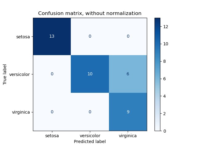
Visualizing Confusion Matrix with ConfusionMatrixDisplay

While the numerical confusion matrix is informative, visualizing it can provide a more intuitive understanding. Scikit-learn’s ConfusionMatrixDisplay class is designed for this purpose.

from sklearn.metrics import ConfusionMatrixDisplay
import matplotlib.pyplot as plt

cm = confusion_matrix(y_true, y_pred) # Compute confusion matrix
disp = ConfusionMatrixDisplay(confusion_matrix=cm, display_labels=labels) # Initialize display
disp.plot() # Plot the confusion matrix
plt.show() # Show the plot

ConfusionMatrixDisplay offers methods like from_estimator and from_predictions to directly create and plot confusion matrices from estimators or pre-calculated predictions, streamlining the visualization process.

An example of a visualized confusion matrix using ConfusionMatrixDisplay, enhancing interpretability.

Conclusion

The scikit-learn confusion matrix is an indispensable tool in your machine learning evaluation toolkit. It provides a detailed breakdown of your classification model’s performance, going beyond simple accuracy to reveal the types of errors your model is making. By understanding how to compute, customize, and visualize confusion matrices using scikit-learn, you gain valuable insights for model improvement and a deeper comprehension of your model’s strengths and weaknesses. Embrace the confusion matrix to become a more effective machine learning practitioner.

References:

• Wikipedia entry for the Confusion matrix
• Scikit-learn User Guide on Model Evaluation